Codanics

Mean

Mean in statistics

The Mean: Unlocking the Power of Averages in Data Science šŸ“ŠšŸŒ

Greetings, Data Explorers! Today, letā€™s delve into the fascinating world of the Mean, a concept thatā€™s as fundamental as it is powerful in the realms of statistics and data science. The Mean, often referred to as the average, is more than just a basic arithmetic tool; itā€™s a key to unlocking insights hidden in data. šŸš€

What is the Mean? šŸ¤”

The Mean, in its simplest form, is the average of a set of numbers. Itā€™s calculated by adding all the numbers together and then dividing by the count of those numbers. Think of it as a way to find the balance point or the center of gravity in a dataset.

The Significance of the Mean in Data Analysis šŸŒŸ

  • A Snapshot of Data: The mean gives a quick snapshot of the data, providing an overall sense of where values lie.
  • Foundation for Further Analysis: Many statistical methods and analyses, such as standard deviation and regression analysis, rely on the mean.
  • Comparative Analysis: The mean is essential for comparing different sets of data, offering a common ground for comparison.

Real-Life Applications of the Mean šŸ¢šŸ“ˆ

  • Business Insights: Companies use the mean to analyze average sales, customer ratings, and other key performance metrics.
  • Educational Performance: Schools and colleges calculate the mean to assess average scores in exams, tests, or overall academic performance.
  • Medical Research: The mean is used to analyze clinical trial results, like average reduction in symptoms or average increase in survival rates.

Calculating the Mean: The Process šŸ§®

The formula for calculating the mean is:

\[ \text{Mean} = \frac{\sum_{i=1}^{n} x_i}{n} \]Ā 

    • Mean: This is what youā€™re trying to find, the average of the numbers.
    • \( \sum \): This is the Greek capital letter sigma, which is used to denote a sum in mathematics.
    • \( \sum_{i=1}^{n} \): This tells you to sum up a series of numbers. The \( i=1 \) at the bottom of the sigma means you start with the first number in your series, and the \( n \) at the top means you continue adding up through the \( n \)th number.
    • \( x_i \): This represents each number in your data set. The \( i \) is an index that goes from 1 to \( n \), so \( x_i \) represents each individual number in the sequence.
    • \( n \): This is the total number of values in your data set.

For example, in a dataset [4, 8, 15, 16, 23, 42], the mean is 4+8+15+16+23+426=18.

Types of Mean

In statistics and data science, the term ā€œmeanā€ typically refers to several different types, each providing unique insights into a dataset. Understanding these variations is crucial for accurately interpreting and analyzing data. Letā€™s explore the most common types of mean:

1. Arithmetic Mean

  • Definition: The most common type of mean, itā€™s calculated by summing up all the values in a dataset and then dividing by the number of values.
  • Formula: \( \text{Arithmetic Mean} = \frac{\sum_{i=1}^{n} x_i}{n} \)
  • Usage: Ideal for interval and ratio data, and when data is evenly distributed without extreme outliers.
  • Example: Calculating the average income of a group of individuals.
  • Consider the dataset: [5, 10, 15, 20, 25]
    • \( \text{Arithmetic Mean} = \frac{5 + 10 + 15 + 20 + 25}{5} = \frac{75}{5} = 15 \)

2. Geometric Mean

  • Definition: The geometric mean is calculated by multiplying all the values together and then taking the nth root (where n is the number of values).
  • Formula: \( \text{Geometric Mean} = (\prod_{i=1}^{n} x_i)^{\frac{1}{n}} \)
  • Usage: Used for datasets that contain values with different ranges or units, such as growth rates.
  • Example: Calculating average growth rates in finance or biology.
  • Consider growth rates: [1.05, 1.08, 1.07]
    • \( \text{Geometric Mean} = (1.05 \times 1.08 \times 1.07)^{\frac{1}{3}} \approx 1.0667 \)
    • The average growth rate is approximately 1.0667 or 6.67%.

3. Harmonic Mean

  • Definition: The harmonic mean is the reciprocal of the arithmetic mean of the reciprocals of the values.
  • Formula: \( \text{Harmonic Mean} = \frac{n}{\sum_{i=1}^{n} \frac{1}{x_i}} \)
  • Usage: Suitable for rates and ratios, like speeds or productivity measurements.
  • Example: Calculating the average speed of a round trip made at different speeds.
  • Consider speeds (km/h): [40, 60, 80]
    • \( \text{Harmonic Mean} = \frac{3}{\frac{1}{40} + \frac{1}{60} + \frac{1}{80}} \approx 53.33 \)
    • The harmonic mean speed is approximately 53.33 km/h.

4. Weighted Mean

  • Definition: The weighted mean takes into account the weight or importance of each value in the dataset.
  • Formula: \( \text{Weighted Mean} = \frac{\sum_{i=1}^{n} w_i x_i}{\sum_{i=1}^{n} w_i} \)
  • Usage: Used when certain values in a dataset are more significant than others.
  • Example: Calculating a studentā€™s grade point average (GPA), where each course has a different credit weight.
  • Consider exam scores: [80, 90, 70] with weights (percentage of total grade): [50%, 25%, 25%]
    • \( \text{Weighted Mean} = \frac{0.5 \times 80 + 0.25 \times 90 + 0.25 \times 70}{0.5 + 0.25 + 0.25} = \frac{40 + 22.5 + 17.5}{1} = 80 \)Ā 
    • The weighted mean score is 80.

5. Truncated (or Trimmed) Mean

  • Definition: The truncated mean involves removing a certain percentage of the smallest and largest values before calculating the mean.
  • Usage: Helpful in reducing the impact of outliers or extreme values.
  • Example: Analyzing data such as income or property values, where extreme values can skew the results.
  • Consider the dataset: [1, 2, 3, 4, 5, 6, 7, 8, 9, 10] and we truncate 10% from each end.
    • Remove the top 10% (1 value) and bottom 10% (1 value): [2, 3, 4, 5, 6, 7, 8, 9]
    • \( \text{Truncated Mean} = \frac{2 + 3 + 4 + 5 + 6 + 7 + 8 + 9}{8} = \frac{44}{8} = 5.5 \)

Each type of mean provides different insights and is appropriate for different types of data and analytical scenarios. Choosing the right mean is essential for accurate data analysis, ensuring that the conclusions drawn are reflective of the underlying data characteristics.

We can use Python to raw plots, here isthe code:

				
					import matplotlib.pyplot as plt
import numpy as np
from scipy import stats

# Data for the example
data = np.array([5, 10, 15, 20, 25])

# Calculating different means
arithmetic_mean = np.mean(data)
geometric_mean = stats.gmean(data)
harmonic_mean = stats.hmean(data)

# Plotting the data and the means
plt.figure(figsize=(10, 6))
plt.bar(range(len(data)), data, color='lightblue', label='Data Points')
plt.axhline(arithmetic_mean, color='red', linestyle='dashed', label=f'Arithmetic Mean: {arithmetic_mean}')
plt.axhline(geometric_mean, color='green', linestyle='dashed', label=f'Geometric Mean: {geometric_mean:.2f}')
plt.axhline(harmonic_mean, color='purple', linestyle='dashed', label=f'Harmonic Mean: {harmonic_mean:.2f}')

plt.xlabel('Data Index')
plt.ylabel('Values')
plt.title('Different Types of Means')
plt.legend()
plt.show()


mean in python
Hereā€™s a graph representing the different types of means for a given dataset:
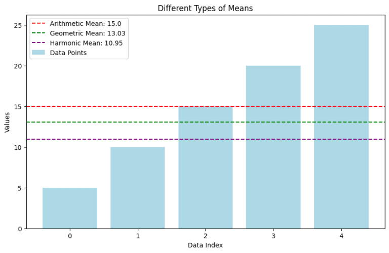
  • Data Points (Light Blue Bars): These bars represent the individual values in the dataset: [5, 10, 15, 20, 25].
  • Arithmetic Mean (Red Dashed Line): This line indicates the arithmetic mean of the dataset. Itā€™s calculated as the sum of all values divided by the number of values.
  • Geometric Mean (Green Dashed Line): This line shows the geometric mean, which is particularly useful for datasets that involve rates and ratios.
  • Harmonic Mean (Purple Dashed Line): The harmonic mean is depicted here, ideal for datasets with rates, such as speeds.

The graph visually demonstrates how each type of mean provides a different perspective on the central tendency of the data, highlighting the importance of choosing the right mean for your specific data analysis needs.

The Mean in Visual Representation šŸ“Š

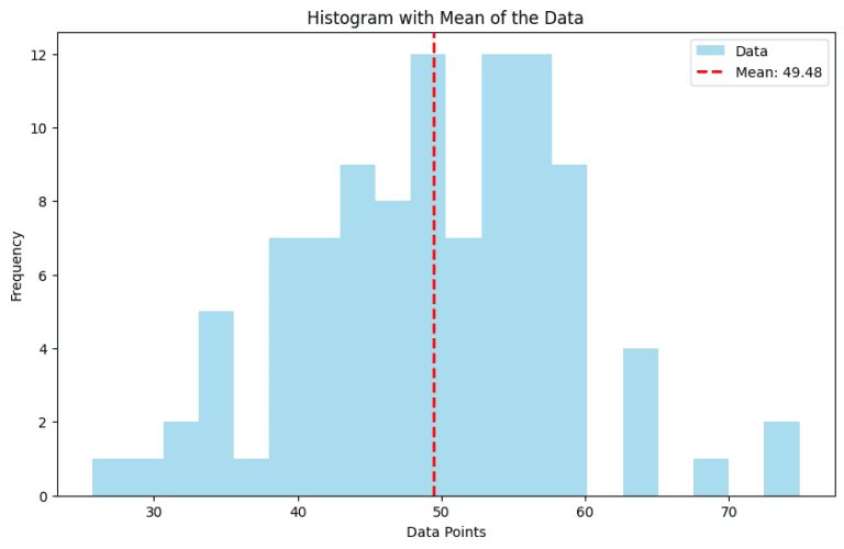
In graphical terms, the mean can be depicted as a line across a bar chart or a dot on a line graph, representing the average value across the dataset.

The Limitations of the Mean šŸš§

While the mean is incredibly useful, itā€™s important to be aware of its limitations:

  • Sensitive to Outliers: Extreme values can skew the mean, making it unrepresentative of the dataset.
  • Not Always the Full Story: The mean might not accurately reflect the distribution of data, especially in skewed distributions.

Conclusion: The Power and Versatility of the Mean šŸš€

In the toolbox of data science, the mean is a versatile and powerful instrument, critical for understanding and interpreting data. Whether youā€™re a seasoned data scientist or a beginner, mastering the mean is a step toward uncovering the stories hidden within numbers.

Remember, the mean is more than just an average; itā€™s a bridge to insights, a guide in a sea of data, and a fundamental pillar in the world of statistics and data science. šŸŒŸšŸ“ˆ

Exit mobile version