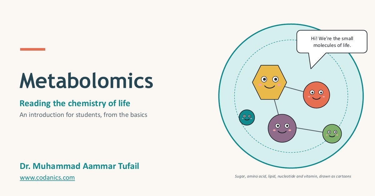
Bioinformatics · Omics · Data analysis Metabolomics: The Complete Guide, from Basics to Data Analysis Learn what metabolites are, how a metabolomics study works from sample to biology, how LC-MS, GC-MS and NMR detect small molecules, and how to process, analyse and interpret the data, with slides, infographics, Python code, key papers and a free video course in Urdu/Hindi. By Dr. Muhammad Aammar TufailCodanicsUpdated 8 November 2026About 35 min read + 4 videos Watch the free video course The short answerMetabolomics reads the chemistry of life. It measures the small molecules (metabolites, usually below 1,500 Da) in a cell, tissue or body fluid, which makes it the omics layer closest to the phenotype. A study follows eight steps: ask a question, design the study, collect and quench samples, extract, measure with LC-MS, GC-MS or NMR, process raw signals into a feature table, run statistics and identify metabolites, and interpret the changes on metabolic pathways. Remember the golden rule: a detected feature is not a confirmed metabolite. ~218Kmetabolite entries in HMDB 5.0 <1,500daltons: how small a metabolite is 8steps in every metabolomics study 4free videos in Urdu/Hindi Key facts: metabolomics at a glance What it measuresSmall molecules: sugars, amino acids, lipids, nucleotides, organic acids, drugs and other xenobiotics StrategiesUntargeted (discover, thousands of signals) and targeted (measure a known panel exactly) Main instrumentsLC-MS, GC-MS and NMR spectroscopy Core dataA feature table: samples × features (m/z at a retention time) × intensity Key statisticsPCA, PLS-DA, t-test or Mann–Whitney with FDR correction, volcano plots Free softwareMZmine, MS-DIAL, XCMS, MetaboAnalyst, SIRIUS, GNPS, Python and R Golden ruleReport the identification confidence level: a detected feature is not a confirmed metabolite Course · Bioinformatics ka ChillaWant to become a bioinformatician? Join Bioinformatics ka Chilla.My complete, practical bioinformatics course in Urdu/Hindi takes you from the basics to real omics data analysis, step by step, with projects you can show in your CV.Biology and computing foundations for beginnersPython and R for biological dataOmics data analysis, including metabolomics workflowsProjects, guidance and a community of learnersRegister for Bioinformatics ka Chilla → When I teach metabolomics, I start with a simple picture: genes tell you what could happen, proteins do the work, but metabolites show what is happening right now. A blood sample from someone who just drank coffee, fasted overnight or took paracetamol tells a different chemical story, even though their genome has not changed. That is why metabolomics has become one of the most exciting, and most in-demand, skills in biology, medicine and agriculture. It is also a field where beginners get lost quickly: m/z, retention time, adducts, features, PQN, PLS-DA, MSI levels. So I built this guide from the slides and infographics I use in class and from my new Metabolomics Complete Course on YouTube. It goes from "what is a metabolite?" all the way to a working Python data-analysis pipeline, in plain English, with every important claim linked to its source. If you are new to the field, read my article on why learning bioinformatics is essential first, then come back here. If you already work in a lab, jump straight to study design and quality control or statistics. Infographic 1: strategies, key terms and the practical workflow. Click to open full size. Infographic 2: the metabolomics workflow, from samples to insight. Click to open full size. Follow me for bioinformatics and research tipsNew lessons on omics, data analysis and scientific research every week.FacebookInstagramTikTokLinkedInGitHubKaggleGoogle ScholarResearchGateYouTubeWhatsApp In this guide What is metabolomics? Metabolites and the metabolome A short history and the growing metabolome Targeted vs untargeted metabolomics The eight-step metabolomics workflow Study design, sample preparation and quality control How LC-MS, GC-MS and NMR detect metabolites Data processing: from raw signals to a feature table Statistics: PCA, PLS-DA, volcano plots (with Python) Metabolite identification and confidence levels Pathway analysis: turning molecules into biology Real-world applications Challenges, frontiers and multi-omics Your learning roadmap The free video course Key papers Tools and databases Glossary FAQ Section 1What is metabolomics? Metabolites and the metabolome Quick answerMetabolites are the small molecules a cell makes, uses or takes in, usually smaller than about 1,500 daltons: sugars, amino acids, lipids, nucleotides, organic acids, vitamins, and foreign chemicals such as drugs. The metabolome is the complete set of metabolites in a sample at one moment, and metabolomics is the large-scale study of it. Because metabolites react to genes, diet, drugs, microbes and environment, the metabolome is the omics layer closest to the phenotype. How small is "small"? A typical enzyme weighs around 50,000 daltons (Da); glucose weighs 180 Da. Metabolites are the inputs, intermediates and outputs of the cell's chemical reactions: glucose is broken down to pyruvate, pyruvate becomes lactate or enters the TCA cycle, and so on. Metabolites are tiny compared with proteins. Sources: Wishart et al., HMDB 5.0, 2022; Liu & Locasale, 2017. ClassExamplesWhy they matter Sugarsglucose, fructoseEnergy and building blocks Amino acidsglutamine, leucine, phenylalanineProtein building blocks, signalling, disease markers Lipidscholesterol, fatty acids, phospholipidsMembranes, energy storage, hormones (studied in lipidomics) NucleotidesATP, NAD⁺Energy currency and redox cofactors Organic acidscitrate, lactate, succinateCentral metabolism (glycolysis, TCA cycle) Xenobioticscaffeine, drugs, pesticidesExposure, drug metabolism, toxicology Why the metabolome is closest to the phenotype Think of the "omics cascade". The genome says what can happen, the transcriptome what the cell plans to do, and the proteome what does the work. The metabolome shows what is happening now, so it tracks traits and health most closely. Oliver Fiehn called metabolomics "the link between genotypes and phenotypes" (Plant Molecular Biology, 2002). The omics cascade: diet, drugs, gut microbes and environment change metabolites directly. Sources: Fiehn 2002; Patti, Yanes & Siuzdak 2012. Your metabolome mixes chemistry from five sources Not every molecule in your blood was made by your own cells. The human metabolome combines chemistry from your cells (glucose, lactate, cholesterol), food (vitamins, plant polyphenols), gut microbes (short-chain fatty acids, TMAO), drugs (paracetamol and its breakdown products) and the environment (pollutants, pesticides, plastics). Everything outside your genes that you are exposed to over a lifetime is called the exposome. Five sources, one metabolome. Sources: Wishart et al., HMDB 5.0, 2022; Johnson, Ivanisevic & Siuzdak, 2016. Start the video course here. In episode 1 I explain these basics in Urdu/Hindi, with examples from biology and disease research: Episode 1 · 21:3301: Introduction to Metabolomics | Basics to Advanced 🧬 | Bioinformatics. Episode 1 of the Metabolomics Complete Course: what metabolomics is and why it matters. Key takeawaysMetabolites are small molecules, usually below 1,500 Da.The metabolome is the full set of metabolites at one moment.It is the omics layer closest to the phenotype and reacts to diet, drugs, microbes and environment. ↑ Back to topNext: A short history of metabolomics → Section 2How did metabolomics grow into a major omics field? Quick answerMetabolomics went mainstream in about 25 years. The term metabonomics was coined in 1999 for NMR studies of body fluids, metabolomics was framed as the link from genotype to phenotype in 2002, the Human Metabolome Database launched with 2,180 metabolites in 2007 alongside the first reporting standards, and by 2022 HMDB 5.0 listed about 218,000 entries. Today the frontier is single-cell, spatial and population-scale metabolomics. 1999"Metabonomics" is coined for NMR studies of metabolic responses in body fluids (Nicholson, Lindon & Holmes, Xenobiotica). 2002The link from genotype to phenotype: Fiehn frames metabolomics as the missing layer (Plant Mol Biol). 2007HMDB launches with 2,180 metabolites, and the Metabolomics Standards Initiative proposes the first reporting standards (Sumner et al.). 2012"The apogee of the omics trilogy" (Patti, Yanes & Siuzdak, Nat Rev Mol Cell Biol). 2016Beyond biomarkers, towards mechanisms (Johnson et al.). 2021Community guide to MS best practice for annotation, quantification and reporting (Alseekh et al., Nat Methods). 2022HMDB 5.0 lists about 218,000 entries (Wishart et al., NAR). TodaySingle-cell, spatial and population-scale studies, and AI tools that predict structures from MS/MS spectra. The human metabolome catalogue grew 100× in 15 yearsMetabolite entries in the Human Metabolome Database, by release year 2.2K6.4K40.2K114.1K217.9K20072009201320182022 Reality check: a big catalogue does not mean we can measure everything. A typical study identifies only a few hundred metabolites, and most detected signals stay unnamed. Identification is still the field's biggest open problem (see Section 12). Source: Wishart et al., HMDB 5.0. Key takeawaysFrom NMR metabonomics in 1999 to a mainstream omics field today.HMDB grew from 2,180 to about 218,000 entries between 2007 and 2022.Most detected signals are still unidentified. ↑ Back to topNext: Targeted vs untargeted → Section 3What is the difference between targeted and untargeted metabolomics? Quick answerTargeted metabolomics measures a predefined list of known metabolites, usually tens to a few hundred, with exact concentrations using pure standards; it is best for testing a hypothesis. Untargeted metabolomics scans widely, detecting thousands of signals as relative amounts, many of them unknown; it is best for discovering new hypotheses. Many labs do both: discover with untargeted, then confirm with targeted. Targeted tests a known list; untargeted scans widely. Sources: Patti et al. 2012; Alseekh et al. 2021. TargetedUntargeted GoalTest a hypothesisDiscover new hypotheses MetabolitesTens to a few hundred, all knownThousands of signals, many unknown AmountsAbsolute (exact concentrations with standards)Relative (fold changes between groups) Typical MSTriple quadrupole, MRM modeHigh-resolution (Orbitrap, Q-TOF) Data analysisSimpler: a clean concentration tableComplex: peak picking, alignment, annotation Main riskMissing what you did not look forFalse discoveries and unidentified features Also good to know: semi-targeted methods measure a large list of known compounds without full absolute quantification; lipidomics focuses on lipids; and fluxomics uses isotope-labelled tracers (for example ¹³C-glucose) to measure how fast metabolites flow through pathways, not just how much is there. Key takeawaysTargeted: known list, exact amounts, hypothesis testing.Untargeted: wide scan, relative amounts, discovery.The strongest studies discover untargeted and confirm targeted. ↑ Back to topNext: The eight-step workflow → Section 4What are the steps of a metabolomics study? Quick answerEvery metabolomics study follows the same eight steps in three phases. Plan: ask a clear question and design the study. Wet lab: collect and quench samples, extract the metabolites and measure them with LC-MS, GC-MS or NMR. Dry lab: process raw signals into a feature table, run statistics and identify the molecules, then interpret the results on pathways and validate key findings. PlanAsk a questione.g. does drug X change liver metabolism?PlanDesign the studygroups, controls, biological replicates, random run orderWet labCollect and quenchfreeze fast so enzymes stop workingWet labExtractsolvents pull metabolites out of the sampleWet labMeasureLC-MS, GC-MS or NMR, with blanks and QCsDry labProcess dataraw signals become a feature tableDry labAnalyze and identifystatistics, then name the moleculesDry labInterpretmap to pathways; validate; form new hypotheses The same eight steps, from question to biology. Adapted from Johnson et al. 2016 and Alseekh et al. 2021. In episode 3 of the course I walk through this whole workflow in detail, including the dry-lab pipeline step by step. If you plan to process your own raw data, this is your roadmap: Episode 3 · 1:05:3803: Complete Metabolomics Workflow & Data Analysis | MS & NMR Guide. Episode 3: the complete metabolomics workflow and data analysis, with MS and NMR (1 hour). Key takeawaysPlan → wet lab → dry lab: eight steps in total.Mistakes in planning cannot be fixed by software later.The dry lab (steps 6–8) is where bioinformaticians create the most value. Course · Bioinformatics ka ChillaLearn the dry lab properly in Bioinformatics ka ChillaSteps 6 to 8 are pure bioinformatics: data processing, statistics, annotation and interpretation. Bioinformatics ka Chilla gives you the programming and analysis skills to do them with confidence.Join the course → ↑ Back to topNext: Study design and quality control → Section 5How do you design a metabolomics study and control data quality? Quick answerData quality is decided before the instrument runs. Use biological replicates in every group, randomize the run order so instrument drift cannot pose as biology, quench metabolism fast with liquid nitrogen or cold solvent, extract every sample the same way, and include pooled QC samples, internal standards and blanks. Record metadata such as fasting state, time of sampling and storage, because metabolites change quickly. Six rules decided before the instrument runs. Source: Alseekh et al., Nature Methods 2021. Your study-design checklist One clear question and a defined comparison (for example treated vs control, disease vs healthy, time course). Biological replicates in every group, not only repeat injections of one sample. Use pilot data or a power analysis to choose the number. Control confounders: match age, sex, diet, fasting state and time of sampling, or record them for statistics. Randomize the run order, and the extraction order, so drift and batch effects are not confused with groups. Plan QC samples: a pooled QC every 5–10 injections, internal standards in every sample, extraction and solvent blanks. Write down everything: sample collection, storage, freeze–thaw cycles and instrument settings. You will need it for reporting. Sample types and how to handle them SampleTips Blood plasma or serumChoose one and use it for all samples; standardize fasting and clotting time; process quickly and store at −80 °C UrineStrong dilution differences between samples: normalize to creatinine, osmolality or with PQN TissueSnap-freeze in liquid nitrogen within seconds; record the wet or dry weight for normalization CellsWash quickly, quench with cold solvent, normalize to cell number or protein content Plants and microbesMetabolism is fast: quench immediately; freeze-dry plant tissue for stable storage Quenching and extractionEnzymes keep working after sampling, so some metabolites (for example ATP or glucose-6-phosphate) change within seconds. Quenching stops metabolism with liquid nitrogen or cold solvent. Extraction then pulls the metabolites out: cold methanol, acetonitrile or methanol–water mixtures for polar metabolites, and two-phase methods (for example with chloroform or MTBE) to separate polar metabolites from lipids. Whatever you choose, extract every sample the same way, in random order. Most common beginner mistake: running all controls first and all treated samples afterwards. The instrument signal drifts over hours, so the "difference" you find may be the instrument, not the biology. Always randomize, and use pooled QCs to prove it. Key takeawaysBiological replicates and randomization are not optional.Quench fast; extract consistently.Pooled QCs, internal standards and blanks make your data trustworthy. ↑ Back to topNext: How the instruments work → Section 6How do mass spectrometry and NMR detect metabolites? Quick answerMass spectrometry weighs molecules as charged ions: a chromatography column (LC or GC) first separates the mixture, an ion source such as electrospray gives each molecule a charge, a mass analyzer sorts the ions by mass-to-charge ratio (m/z), and a detector counts them. MS/MS fragments an ion to fingerprint its structure. NMR instead measures how atomic nuclei, usually ¹H, absorb radio waves in a strong magnet; it detects fewer metabolites but is highly reproducible, quantitative and non-destructive. Mass spectrometry in five steps. Sources: Patti et al. 2012; Alseekh et al. 2021. Masses from HMDB. PlatformBest forNotes LC-MSMost metabolites: polar and non-polar, lipidsReversed-phase (RP) columns for less polar compounds, HILIC for very polar ones; run positive and negative ionization modes GC-MSSmall, volatile or derivatized compounds: organic acids, sugars, amino acidsVery reproducible spectra and large libraries (e.g. NIST); needs chemical derivatization for many metabolites NMRAbundant metabolites; absolute quantification; structureNon-destructive and very reproducible, but less sensitive (µM range) CE-MSCharged, highly polar metabolitesCapillary electrophoresis needs very small sample volumes m/z and adducts: why one molecule gives several signals m/z means mass divided by charge. Most metabolite ions carry a single charge, so m/z is the molecule's mass plus or minus a proton, or plus another ion (an adduct) such as Na⁺, K⁺ or NH₄⁺. Glucose (monoisotopic mass 180.0634 Da) appears at m/z 179.0561 as [M−H]⁻ in negative mode and at 203.0526 as [M+Na]⁺ in positive mode. This short script calculates the common ions and matches an observed m/z within a ppm tolerance: mz_calculator.pyCopy# mz_calculator.py: which m/z values will a metabolite give in the mass spectrometer? # No extra packages needed (standard Python 3). PROTON = 1.007276 # mass of a proton (Da) NA = 22.989218 # Na+ ion K = 38.963158 # K+ ion NH4 = 18.033823 # NH4+ ion # Monoisotopic masses (Da) from HMDB METABOLITES = { "glucose": 180.063388, "phenylalanine": 165.078979, "lactate (lactic acid)": 90.031694, "citrate (citric acid)": 192.027003, "glutamine": 146.069142, } def adducts(m): """Common single-charge ions for a neutral mass m.""" return { "[M+H]+": m + PROTON, "[M+Na]+": m + NA, "[M+K]+": m + K, "[M+NH4]+": m + NH4, "[M-H]-": m - PROTON, } def ppm_error(observed, theoretical): """Mass error in parts per million (ppm).""" return (observed - theoretical) / theoretical * 1e6 def match(observed_mz, tolerance_ppm=5): """Find which metabolite/adduct could explain an observed m/z.""" hits = [] for name, mass in METABOLITES.items(): for ion, mz in adducts(mass).items(): err = ppm_error(observed_mz, mz) if abs(err) <= tolerance_ppm: hits.append((name, ion, round(mz, 4), round(err, 2))) return hits if __name__ == "__main__": for name, mass in METABOLITES.items(): ions = ", ".join(f"{ion} {mz:.4f}" for ion, mz in adducts(mass).items()) print(f"{name:22s} M = {mass:.4f} -> {ions}") print() for observed in [179.0560, 166.0864, 203.0530]: print(f"Observed m/z {observed}: {match(observed) or 'no match within 5 ppm'}") TerminalCopypython mz_calculator.py Result: for every metabolite, the five common ions (glucose: [M+H]⁺ 181.0707, [M+Na]⁺ 203.0526, [M−H]⁻ 179.0561), then the matches: m/z 179.0560 → glucose [M−H]⁻ (−0.63 ppm), 166.0864 → phenylalanine [M+H]⁺ (0.87 ppm), 203.0530 → glucose [M+Na]⁺ (1.94 ppm). Tested with Python 3.13. Mass alone is not identity. Glucose, fructose and galactose have exactly the same mass (they are isomers). You need retention time, MS/MS spectra or a reference standard to tell them apart. MS/MS: fragment patterns fingerprint a moleculeIn tandem mass spectrometry, the instrument picks one ion (the precursor), smashes it by collision with gas (CID) and records the fragments. Phenylalanine [M+H]⁺ at m/z 166.09 loses formic acid (−46) to give 120.08, and also produces a ring fragment at 91.05. The same fragments plus the same mass are strong evidence of identity. In untargeted work, instruments collect MS/MS automatically, either for the most intense ions (DDA, data-dependent acquisition) or for all ions in wide windows (DIA, data-independent acquisition). MS/MS spectrum of phenylalanine (simplified for teaching). Fragment masses from HMDB and MoNA reference spectra. MS or NMR? MS detects more molecules; NMR is more reproducible. Typical values. Sources: Emwas et al. 2019; Patti et al. 2012; Alseekh et al. 2021. Key takeawaysLC-MS detects the most metabolites; GC-MS and NMR have their own strengths.One metabolite gives several ions (adducts, isotopes): mass alone is not identity.MS/MS fragments are the fingerprint that supports identification. ↑ Back to topNext: Data processing → Section 7How is raw metabolomics data processed into a feature table? Quick answerProcessing software turns raw instrument files into a feature table in four main steps: peak picking finds every signal, alignment matches the same peak across samples despite small retention-time shifts, cleaning fills gaps and removes noise, blank signals and unstable features, and normalization corrects for drift and dilution. Free tools such as MZmine, MS-DIAL and XCMS do this. The result is a table of samples by features, where a feature is one m/z at one retention time. From raw traces to a feature table. Common free software: XCMS, MZmine, MS-DIAL. Sources: Alseekh et al. 2021; Johnson et al. 2016. The processing pipeline, step by step Convert files from the vendor format to open mzML with ProteoWizard msConvert (MS-DIAL also reads many vendor files directly). Peak picking: detect chromatographic peaks for every m/z in every sample. Alignment: match the same feature across samples and correct retention-time shifts. Gap filling: go back to the raw data to recover peaks missed in some samples. Grouping: link isotopes, adducts and in-source fragments that belong to one compound (e.g. CAMERA, MS-DIAL, MZmine ion identity networking). Filtering: remove features found in blanks (e.g. sample/blank ratio below 3), missing in most samples, or unstable in pooled QCs (RSD above 20–30%). Drift and batch correction: model the QC signal over the run order (e.g. LOESS-based QC-RSC) and correct every feature. Normalization, transformation and scaling: correct dilution (PQN, internal standards, creatinine for urine), log-transform, then scale (Pareto or autoscaling) for multivariate statistics. ToolWhat it doesCost MZmineLC-MS and GC-MS processing with a graphical interface; ion identity networking; export to GNPS and SIRIUSFree, open source MS-DIALDDA and DIA processing, built-in spectral libraries, lipidomicsFree XCMSR/Bioconductor package for peak picking, alignment and groupingFree, open source MetaboAnalystWeb platform for statistics, enrichment and pathway analysis, and raw-spectra processingFree Vendor softwaree.g. Compound Discoverer, Progenesis QI, MassHunterCommercial NMR toolse.g. NMRProcFlow (free) for spectra processing, Chenomx for quantificationFree / commercial In episode 4, a one-minute summary, I list the core tasks a bioinformatician owns in a metabolomics project: Episode 4 · 0:5904: Metabolomics Data Analysis Tasks for Bioinformaticians 💻🧬. Episode 4: the data-analysis tasks of a bioinformatician in metabolomics. Key takeawaysPeak picking → alignment → cleaning → normalization.Use pooled QCs and blanks to filter unreliable features.A feature is a signal, not yet a named metabolite. ↑ Back to topNext: Statistics with Python → Section 8Which statistics are used in metabolomics, and how do you run them in Python? Quick answerStart unsupervised with PCA to see groups, trends and outliers, and check that pooled QCs cluster tightly. Then test each feature with a t-test, Welch test or Mann–Whitney test on log-transformed data and correct for multiple testing with the Benjamini–Hochberg false discovery rate. Show results in a volcano plot of fold change against significance. Supervised models such as PLS-DA can rank features by VIP score, but they overfit easily and must be validated with cross-validation and permutation tests. PCA shows samples; the volcano plot shows features. Illustrative data. Free tool: MetaboAnalyst (Pang et al. 2024). MethodQuestion it answersWatch out for PCADo samples group? Are there outliers or batch effects? Do QCs cluster?Unsupervised: groups may not separate even when real differences exist PLS-DA / OPLS-DAWhich features best separate known groups (VIP scores)?Overfits easily: report cross-validated Q² and a permutation test t-test / Welch / Mann–WhitneyIs this feature different between two groups?Thousands of tests: always correct with FDR ANOVA / Kruskal–WallisDifferences among three or more groupsFollow with post-hoc tests Fold changeHow big is the change?Combine with significance: big but noisy is not reliable Random forest, ROC curvesCan a biomarker panel classify new samples?Validate on an independent cohort A complete pipeline in PythonThese two scripts let you practise without your own data. The first makes a realistic example feature table (22 samples: 8 control, 8 treated, 6 pooled QCs; 300 features, of which 30 really change). The second runs the full pipeline: missing-value filter, imputation, QC-RSD filter, PQN normalization, log transformation, Pareto scaling, PCA, Welch t-tests with FDR, and a volcano plot. To use your own data, export a CSV with the same layout from MZmine, MS-DIAL or XCMS. make_example_data.pyCopy# make_example_data.py: create a realistic example feature table to practise on # pip install numpy pandas import numpy as np import pandas as pd rng = np.random.default_rng(42) n_features, n_per_group, n_qc = 300, 8, 6 # each feature gets a typical intensity (log-normal, like real LC-MS data) base = rng.lognormal(mean=10, sigma=1.2, size=n_features) effect = np.ones(n_features) effect[:15] = rng.uniform(2.0, 4.0, 15) # 15 features go UP in treated samples effect[15:30] = rng.uniform(0.25, 0.5, 15) # 15 features go DOWN def samples(n, fold, noise=0.25): return base * fold * rng.lognormal(0, noise, size=(n, n_features)) control = samples(n_per_group, 1.0) treated = samples(n_per_group, effect) qc = samples(n_qc, (1 + effect) / 2, noise=0.08) # pooled QC = mix of all samples dilution = rng.uniform(0.7, 1.3, size=(2 * n_per_group + n_qc, 1)) # unequal sample amounts X = np.vstack([control, treated, qc]) * dilution X[rng.random(X.shape) < 0.03] = np.nan # a few missing values, as in real data names = [f"C{i+1}" for i in range(n_per_group)] + [f"T{i+1}" for i in range(n_per_group)] + [f"QC{i+1}" for i in range(n_qc)] groups = ["Control"] * n_per_group + ["Treated"] * n_per_group + ["QC"] * n_qc mz = np.round(rng.uniform(70, 900, n_features), 4) rt = np.round(rng.uniform(0.5, 15, n_features), 2) cols = [f"{m}_{r}" for m, r in zip(mz, rt)] # feature name = m/z_retention time df = pd.DataFrame(X, columns=cols) df.insert(0, "group", groups) df.insert(0, "sample", names) df.to_csv("feature_table.csv", index=False) print(f"Saved feature_table.csv: {df.shape[0]} samples x {n_features} features") metabolomics_stats.pyCopy# metabolomics_stats.py: from a feature table to PCA, statistics and a volcano plot # pip install numpy pandas scipy scikit-learn matplotlib # Input: feature_table.csv with columns sample, group (Control / Treated / QC), then one column per feature import numpy as np import pandas as pd import matplotlib.pyplot as plt from scipy import stats from sklearn.decomposition import PCA df = pd.read_csv("feature_table.csv") meta, X = df[["sample", "group"]], df.drop(columns=["sample", "group"]) print("Start:", X.shape[1], "features") # 1. Remove features missing in more than half of the samples X = X.loc[:, X.isna().mean() <= 0.5] # 2. Fill the remaining gaps with 1/5 of the feature's smallest value (a common, simple choice) X = X.fillna(X.min() / 5) # 3. Keep features that are stable in the pooled QC samples (RSD below 30%) qc = X[meta.group == "QC"] rsd = qc.std() / qc.mean() * 100 X = X.loc[:, rsd < 30] print("After missing-value and QC-RSD filters:", X.shape[1], "features") # 4. PQN normalization: corrects for samples that are more or less concentrated reference = X[meta.group == "QC"].median() quotients = X.div(reference, axis=1) X = X.div(quotients.median(axis=1), axis=0) # 5. Log-transform (makes intensities more normal), then Pareto-scale for PCA L = np.log2(X) P = (L - L.mean()) / np.sqrt(L.std()) # 6. PCA: do the groups separate? Are the QCs tightly clustered? pca = PCA(n_components=2) scores = pca.fit_transform(P) var = pca.explained_variance_ratio_ * 100 colours = {"Control": "#0072B2", "Treated": "#D55E00", "QC": "#999999"} fig, ax = plt.subplots(figsize=(6, 5)) for g, c in colours.items(): m = (meta.group == g).values ax.scatter(scores[m, 0], scores[m, 1], c=c, label=g, s=60, edgecolor="white") ax.set_xlabel(f"PC1 ({var[0]:.1f}%)") ax.set_ylabel(f"PC2 ({var[1]:.1f}%)") ax.legend(frameon=False) ax.set_title("PCA score plot") fig.tight_layout() fig.savefig("pca.png", dpi=200) # 7. Univariate test per feature: Welch t-test on log data, then FDR correction c, t = L[meta.group == "Control"], L[meta.group == "Treated"] p = stats.ttest_ind(t, c, equal_var=False).pvalue q = stats.false_discovery_control(p, method="bh") # Benjamini-Hochberg log2fc = t.mean() - c.mean() # already in log2 units res = pd.DataFrame({"feature": L.columns, "log2FC": log2fc.values, "p": p, "q_FDR": q}) res["significant"] = (res.q_FDR < 0.05) & (res.log2FC.abs() >= 1) res = res.sort_values("q_FDR") res.to_csv("results.csv", index=False) print("Significant features (FDR < 0.05 and at least 2-fold):", int(res.significant.sum())) print(res.head(5).to_string(index=False)) # 8. Volcano plot fig, ax = plt.subplots(figsize=(6, 5)) col = np.where(~res.significant, "#BBBBBB", np.where(res.log2FC > 0, "#D55E00", "#0072B2")) ax.scatter(res.log2FC, -np.log10(res.p), c=col, s=18) ax.axvline(-1, ls="--", c="grey", lw=0.8) ax.axvline(1, ls="--", c="grey", lw=0.8) ax.set_xlabel("log2 fold change (Treated / Control)") ax.set_ylabel("-log10 p-value") ax.set_title("Volcano plot") fig.tight_layout() fig.savefig("volcano.png", dpi=200) print("Saved pca.png, volcano.png and results.csv") TerminalCopypip install numpy pandas scipy scikit-learn matplotlib python make_example_data.py python metabolomics_stats.py Result: 300 features in, 254 left after the missing-value and QC-RSD filters, and 18 significant features (FDR below 0.05 and at least 2-fold), all of them among the 30 truly changed ones. PCA separates control and treated samples while the six pooled QCs cluster tightly in the centre, which is exactly what a good dataset looks like. Tested on 8 November 2026 with Python 3.13, NumPy 2.2, pandas 2.2, SciPy 1.15, scikit-learn 1.8 and matplotlib 3.10. The two plots the script saves: pca.png and volcano.png. Notice the one treated sample far below the others on PC2: in real data, check outliers like this before removing anything. Prefer R or no code? Upload the same CSV to MetaboAnalyst for point-and-click statistics, or use the MetaboAnalystR package. For R basics, see my course R with Aammar; for Python, Python ka Chilla for data science. Key takeawaysPCA first: check groups, outliers and QC clustering.Univariate tests on log data, always with FDR correction.Validate PLS-DA; never trust a pretty separation alone. ↑ Back to topNext: Metabolite identification → Section 9How are metabolites identified, and what are the confidence levels? Quick answerA feature is identified by combining accurate mass (usually within 5 ppm), isotope pattern, retention time and MS/MS fragmentation, matched against spectral libraries or predicted with in-silico tools. The Metabolomics Standards Initiative defines four confidence levels: level 1 identified with a pure reference standard on at least two properties, level 2 putatively annotated by a library match, level 3 assigned to a compound class, and level 4 unknown. Always report the level. Naming a metabolite comes with a confidence level. Source: Sumner et al. 2007 (MSI); Alseekh et al. 2021. LevelNameEvidence needed 1IdentifiedMatches a pure standard run on the same system on two or more properties (e.g. retention time and MS/MS) 2Putatively annotatedSpectrum matches a library or the literature, without a standard 3Compound classOnly the chemical family is known (e.g. "a phosphatidylcholine") 4UnknownSeen reproducibly, but no identity yet For high-resolution MS, many labs also use the five-level scale of Schymanski et al. (2014), which splits putative structures into finer levels. Databases and tools for annotation HMDB: human metabolites with masses, spectra and biology MassBank and MoNA: open MS/MS reference spectra GNPS: library search and molecular networking that groups related molecules by similar spectra SIRIUS with CSI:FingerID: predicts molecular formulas and structures from MS/MS, even for compounds not in libraries LIPID MAPS: lipid structures and classification PubChem and ChEBI: general chemical databases Do not over-claim. A mass-only match is not even level 2: dozens of compounds can share a mass within 5 ppm. If a metabolite drives your main conclusion, confirm it with a standard (level 1) or with a targeted method. Key takeawaysMass + isotopes + retention time + MS/MS = identification evidence.Report the MSI level for every named metabolite.Confirm your key findings with standards. ↑ Back to topNext: Pathway analysis → Section 10How does pathway analysis turn changed metabolites into biology? Quick answerPathway analysis maps changed metabolites onto known pathways in databases such as KEGG, Reactome and SMPDB, tests whether a pathway contains more changed metabolites than expected by chance (over-representation or enrichment analysis), and looks for where flow is blocked or rerouted. For untargeted data without confident identifications, mummichog-style methods test pathways directly from m/z features. Example: tumor vs normal tissue (simplified, illustrative). Glucose is pushed to lactate even with oxygen present: the Warburg effect. Sources: Johnson et al. 2016; Martínez-Reyes & Chandel 2021. Over-representation analysis (ORA): is the list of significant metabolites enriched in a pathway? Quantitative enrichment (MSEA): uses all measured values, not only a cut-off list Topology analysis: gives more weight to metabolites at important positions in a pathway mummichog / functional analysis: works from m/z features before identification (Li et al., 2013); available in MetaboAnalyst Use the right background. Test enrichment against the metabolites your method can actually measure, not against every metabolite in KEGG. Otherwise central pathways such as amino acid metabolism look "enriched" simply because your platform detects them well. Key takeawaysMap changes onto pathways, then test enrichment.Choose the right background set.Pathways generate hypotheses; experiments confirm them. ↑ Back to topNext: Applications → Section 11Where is metabolomics used in the real world? Quick answerMetabolomics is already used from hospitals to farms: newborn screening for inherited metabolic disorders, predicting type 2 diabetes and many other diseases from blood profiles, discovering oncometabolites in cancer, linking gut-microbe metabolites to heart disease, and guiding crop breeding for better flavour. It is also central to drug discovery, toxicology, nutrition and environmental research. Newborn screeningA heel-prick blood spot is screened by tandem MS for dozens of inherited disorders, such as phenylketonuria (high phenylalanine).Routine in many countries Diabetes riskFive blood amino acids flagged people who developed type 2 diabetes up to 12 years later.Wang TJ et al., Nat Med 2011 CancerMetabolomics revealed 2-hydroxyglutarate, an "oncometabolite" made by mutant IDH1 in brain tumours.Dang et al., Nature 2009 Population healthNMR profiles of about 118,000 UK Biobank adults predicted the risk of 24 conditions.Buergel et al., Nat Med 2022 Gut microbes and the heartTMAO, made from dietary choline by gut microbes, was linked to cardiovascular disease risk.Wang Z et al., Nature 2011 Crops and foodMapping flavour chemicals guided breeding of tastier tomatoes.Tieman et al., Science 2017 Metabolomics from hospitals to farms. See also Wishart, Nat Rev Drug Discov 2016. Key takeawaysClinical use: newborn screening, risk prediction, cancer.Microbiome, nutrition, drugs and toxicology.Agriculture and food quality. ↑ Back to topNext: Challenges and frontiers → Section 12What are the biggest challenges and frontiers in metabolomics? Quick answerThe biggest open problem is unknowns: most detected features still have no name. Other challenges are poor comparability between labs and instruments, metabolites that change within seconds of sampling, and telling cause from effect. The frontiers are single-cell and spatial metabolomics, population-scale studies of 100,000+ people, AI tools that predict structures from MS/MS spectra, and integration with genomics, transcriptomics and proteomics. Open problems and the next tools. Sources: Wishart et al. 2022; Alseekh et al. 2021; Dührkop et al., SIRIUS 4, 2019. Multi-omics integrationMetabolomics becomes even more powerful when combined with other layers: a gene variant (genomics) that changes an enzyme's expression (transcriptomics and proteomics) and so a metabolite level (metabolomics) tells a complete causal story. Methods include correlation networks, joint dimensionality reduction (for example MOFA or DIABLO in mixOmics) and pathway-level integration. For protein structures behind enzymes, see my AlphaFold tutorial. Reporting and sharing your dataGood science is reproducible. Deposit raw data and metadata in MetaboLights or the Metabolomics Workbench, describe your QC procedures, and report identification levels. These repositories are also free sources of real datasets for practice. Key takeawaysUnknowns are the field's biggest problem.Single-cell, spatial, population-scale and AI annotation are the frontiers.Share raw data and report QC and identification levels. ↑ Back to topNext: Your learning roadmap → Section 13How do you learn metabolomics data analysis, step by step? Quick answerLearn in layers: first biochemistry basics and the vocabulary (metabolite, feature, m/z, retention time), then how LC-MS, GC-MS and NMR work, then Python or R and statistics, then hands-on processing with MZmine or MS-DIAL and analysis with MetaboAnalyst on public datasets from MetaboLights or the Metabolomics Workbench. Finish with a small project you can put on GitHub and in your CV. Week 1: concepts. Read Sections 1–4 of this guide and watch episodes 1 and 2 of the video course. Week 2: instruments and workflow. Sections 5–6 and episode 3; read the primer by Liu & Locasale (2017). Week 3: programming and statistics. Run the Python scripts in Section 8; learn pandas, PCA and FDR. Week 4: real data. Download a small study from MetaboLights, process it with MZmine or MS-DIAL, and analyse it in MetaboAnalyst and Python. Week 5: annotation and pathways. Annotate top features with GNPS or SIRIUS, report MSI levels, run pathway analysis. Week 6: portfolio. Write up your project as a GitHub repository and a short report or poster. Episode 2 is the best place to start building your vocabulary before you open any software: Episode 2 · 6:4102: Key Terms in Metabolomics | Essential Vocabulary for Beginners. Episode 2: the key terms you need before reading papers or using MetaboAnalyst. Course · Bioinformatics ka ChillaReady to learn bioinformatics from zero to job-ready?Register for Bioinformatics ka Chilla, my complete course in Urdu/Hindi. Learn the biology, programming and data analysis behind genomics, proteomics and metabolomics with practical projects.Step-by-step lessons for complete beginnersPython, R and statistics for biological dataOmics workflows, including metabolomics data analysisProjects for your CV, PhD and job applicationsRegister for Bioinformatics ka Chilla → Key takeawaysConcepts → instruments → coding and statistics → real data → portfolio.Practise on public MetaboLights and Workbench datasets.A finished project on GitHub beats ten certificates. The free Metabolomics Complete Course (Urdu/Hindi)4 videos so far, in order. New episodes are added to the same playlist. Metabolomics Complete Course: Practical Data AnalysisCodanics on YouTube · Urdu/HindiOpen playlist 01: Introduction to Metabolomics | Basics to Advanced 🧬 | Bioinformatics · 21:3302: Key Terms in Metabolomics | Essential Vocabulary for Beginners · 6:4103: Complete Metabolomics Workflow & Data Analysis | MS & NMR Guide · 1:05:3804: Metabolomics Data Analysis Tasks for Bioinformaticians 💻🧬 · 0:59 Download the slides. The 20 teaching slides used in this guide ("Metabolomics: reading the chemistry of life") are free to download as a PDF for self-study and teaching, with credit to Codanics. Download the slides (PDF, 0.7 MB) → Key papers to readPeer-reviewed reviews, standards and databases cited in this guide Start here: reviews1Liu & Locasale (2017) Metabolomics: a primerTrends in Biochemical Sciences 42:274–2842Patti, Yanes & Siuzdak (2012) Metabolomics: the apogee of the omics trilogyNat Rev Mol Cell Biol 13:263–2693Johnson, Ivanisevic & Siuzdak (2016) Metabolomics: beyond biomarkers and towards mechanismsNat Rev Mol Cell Biol 17:451–4594Rinschen et al. (2019) Identification of bioactive metabolites using activity metabolomicsNat Rev Mol Cell Biol 20:353–3675Wishart (2016) Emerging applications of metabolomics in drug discovery and precision medicineNat Rev Drug Discov 15:473–484 Methods, standards and databases1Alseekh et al. (2021) Mass spectrometry-based metabolomics: a guide for annotation, quantification and best reporting practicesNature Methods 18:747–7562Sumner et al. (2007) Proposed minimum reporting standards for chemical analysisMetabolomics 3:211–2213Schymanski et al. (2014) Identifying small molecules via high resolution mass spectrometry: communicating confidenceEnviron Sci Technol 48:2097–20984Emwas et al. (2019) NMR spectroscopy for metabolomics researchMetabolites 9:1235Wishart et al. (2022) HMDB 5.0: the Human Metabolome Database for 2022Nucleic Acids Research 50:D622–D6316Pang et al. (2024) MetaboAnalyst 6.0Nucleic Acids Research 52:W398–W4067Dührkop et al. (2019) SIRIUS 4: turning tandem mass spectra into metabolite structure informationNature Methods 16:299–3028Li et al. (2013) Predicting network activity from high throughput metabolomics (mummichog)PLoS Comput Biol 9:e1003123 Free tools, databases and data repositories 1HMDBHuman Metabolome Database2MetaboAnalystStatistics and pathway analysis online3MZmineOpen-source LC-MS/GC-MS processing4MS-DIALProcessing with built-in libraries5XCMS (R)Peak picking and alignment in R6GNPSSpectral libraries and molecular networking7SIRIUSFormula and structure prediction from MS/MS8MoNAMassBank of North America spectra9KEGG PathwayMetabolic pathway maps10LIPID MAPSLipid structures and tools11MetaboLightsPublic metabolomics datasets (EMBL-EBI)12Metabolomics WorkbenchPublic datasets and tools (NIH) Related guides and courses on Codanics 1Bioinformatics ka ChillaThe complete bioinformatics course2Why learning bioinformatics is essentialStart here if you are new3AlphaFold tutorialProtein structure prediction4Python ka Chilla for data science40 days of Python for analysis5R with AammarR for statistics and figures6Pandas mastery guideHandle feature tables in Python7Data visualisation guideChoose the right plot8ABC of statisticsStatistics from the basics9Handling outliersSpot and treat outlier samples10Systematic review and meta-analysisSynthesize published evidence11Conference posters with AI toolsPresent your metabolomics results12Using AI tools in scientific writingWrite up your study More research, AI and bioinformatics guides on the Codanics blog. Know someone learning omics or bioinformatics?Share this free guide with your lab group, classmates or students. WhatsApp LinkedIn Facebook X Email Metabolomics glossary30 key terms in plain English MetaboliteA small molecule (usually below about 1,500 Da) that a cell makes, uses or takes in, such as glucose, lactate or an amino acid.MetabolomeThe complete set of metabolites in a biological sample at a given time.MetabolomicsThe large-scale measurement and study of metabolites in biological samples.MetabonomicsAn older, closely related term coined for NMR studies of metabolic responses in body fluids; today used almost interchangeably with metabolomics.LipidomicsA branch of metabolomics that focuses on lipids, such as fatty acids, phospholipids and cholesterol.ExposomeEverything outside your genes that you are exposed to over a lifetime: food, drugs, microbes and pollutants.XenobioticA foreign chemical in the body, such as a drug, food additive or pollutant.Targeted metabolomicsMeasuring a predefined panel of known metabolites, usually with pure standards for exact amounts.Untargeted metabolomicsProfiling as many signals as possible to discover differences, usually as relative amounts.QuenchingStopping metabolism immediately after sampling, for example with liquid nitrogen or cold solvent.Pooled QCA mixture of all study samples, injected throughout the run to monitor and correct instrument drift.Internal standardA known compound (often isotope-labelled) added to every sample to check recovery and correct signal variation.BlankA sample without biological material, used to detect contamination from tubes, solvents and the instrument.m/zMass-to-charge ratio of an ion, the value a mass spectrometer measures.AdductThe ion form of a molecule, such as [M+H]+, [M+Na]+ or [M−H]−.Retention timeWhen a compound comes out (elutes) of the chromatography column.ESIElectrospray ionization: a soft method that turns molecules in liquid into ions for LC-MS.MS/MSTandem mass spectrometry: an ion is selected and broken into fragments whose masses help identify it.FeatureA detected signal (one m/z at one retention time), not yet a confirmed metabolite.Feature tableA matrix with samples in rows, features in columns and intensities in the cells.ppm errorThe difference between measured and theoretical mass in parts per million; high-resolution instruments reach below 5 ppm.PQNProbabilistic quotient normalization: corrects for samples that are more or less diluted.Pareto scalingDividing each centred feature by the square root of its standard deviation, so large and small signals both contribute.PCAPrincipal component analysis: an unsupervised map of samples that shows groups, trends and outliers.PLS-DAPartial least squares discriminant analysis: a supervised model that separates known groups; it must be validated because it overfits easily.VIP scoreVariable importance in projection: ranks features by their contribution to a PLS-DA model.FDRFalse discovery rate: the expected share of false positives among significant results, controlled with the Benjamini–Hochberg method.Volcano plotA plot of fold change against statistical significance for every feature.AnnotationAssigning a putative identity to a feature, with a stated confidence level.Pathway enrichmentTesting whether a metabolic pathway contains more changed metabolites than expected by chance. Frequently asked questions Search the FAQWhat is metabolomics in simple words?Metabolomics is the large-scale study of the small molecules (metabolites) in a cell, tissue, body fluid or organism, such as sugars, amino acids, lipids and organic acids. It shows the chemistry that is happening right now, so it is the omics layer closest to the phenotype.What is the difference between a metabolite and the metabolome?A metabolite is one small molecule, usually below about 1,500 Da, that a cell makes, uses or takes in. The metabolome is the complete set of metabolites in a sample at a given time.What is the difference between targeted and untargeted metabolomics?Targeted metabolomics measures a predefined list of known metabolites, usually tens to a few hundred, with exact amounts using pure standards; it tests a hypothesis. Untargeted metabolomics profiles thousands of signals, many unknown, as relative amounts; it discovers new hypotheses. Many labs discover with untargeted and confirm with targeted.Which instruments are used in metabolomics?Mostly mass spectrometry coupled to liquid chromatography (LC-MS) or gas chromatography (GC-MS), and nuclear magnetic resonance (NMR) spectroscopy. LC-MS detects the most metabolites, GC-MS is strong for small volatile or derivatized compounds, and NMR is highly reproducible, quantitative and non-destructive.Is mass spectrometry or NMR better for metabolomics?Neither is better for everything. Mass spectrometry is far more sensitive and detects hundreds to thousands of metabolites per run. NMR detects fewer (tens to about 100) but is very reproducible, quantifies directly and leaves the sample intact. Large studies often combine both.What is a feature in metabolomics?A feature is one detected signal defined by an m/z value and a retention time, with an intensity in each sample. It is not yet a named metabolite: one metabolite can give several features (adducts, isotopes, fragments), and many features stay unidentified.What does m/z mean?m/z is the mass-to-charge ratio of an ion. Most metabolite ions carry a single charge, so m/z is roughly the molecule's mass plus or minus a proton or another adduct. For example, glucose (180.063 Da) appears at m/z 179.056 as [M−H]− and at m/z 203.053 as [M+Na]+.How are metabolites identified?By matching accurate mass, isotope pattern, retention time and MS/MS fragmentation spectra against databases such as HMDB, MassBank, MoNA, GNPS and METLIN, or with in-silico tools such as SIRIUS. Confirmed identification (level 1) requires matching a pure reference standard on at least two properties.What are the metabolite identification confidence levels?The Metabolomics Standards Initiative defines four levels: level 1 identified (matches a pure standard), level 2 putatively annotated (matches a library spectrum), level 3 compound class, and level 4 unknown. Always report the level for every named metabolite.Which software is used for metabolomics data analysis?Free tools include MZmine, MS-DIAL and XCMS for processing raw LC-MS data, MetaboAnalyst for statistics and pathway analysis, GNPS for molecular networking and SIRIUS for structure annotation. Python and R are used for custom pipelines.Can I learn metabolomics data analysis without a wet lab?Yes. Public datasets from MetaboLights and the Metabolomics Workbench let you practise processing, statistics, annotation and pathway analysis with only a computer. Basic chemistry, statistics and Python or R are the key skills.How many samples do I need for a metabolomics study?It depends on the effect size and variability, but biological replicates in every group are essential, not just repeat injections of one sample. Pilot data or a power analysis help; many discovery studies use at least 6–10 biological replicates per group, and clinical studies far more.What is a pooled QC sample?A pooled QC is made by mixing a small amount of every study sample. It is injected regularly through the run to track instrument drift, filter unreliable features (for example RSD above 30%) and correct batch effects.What is the Human Metabolome Database (HMDB)?HMDB is a free online database of human metabolites with masses, spectra, concentrations and biological information. Version 5.0 (2022) contains about 218,000 metabolite entries, up from 2,180 in 2007.Where can I learn metabolomics in Urdu or Hindi?Watch the free Codanics Metabolomics Complete Course playlist on YouTube and join the Bioinformatics ka Chilla course on codanics.com for a structured, practical path through bioinformatics, including omics data analysis.No questions match. Try another word. Course · Bioinformatics ka ChillaTurn this guide into a skill: join Bioinformatics ka ChillaStructured lessons, practical projects and guidance in Urdu/Hindi, for students, researchers and anyone moving into bioinformatics.Register now → Get bioinformatics and research tips on WhatsAppFollow Codanics on WhatsApp for new lessons, course updates and scholarships.Join on WhatsApp Stay connected with Dr. AammarBioinformatics, data science and research lessons, every week.FacebookInstagramTikTokLinkedInGitHubKaggleGoogle ScholarResearchGateYouTubeWhatsApp About the author. Dr. Muhammad Aammar Tufail is the founder of Codanics and completed his PhD in a Marie Skłodowska-Curie programme. He teaches bioinformatics, data science, AI tools for research and scientific writing in Urdu and Hindi. Follow him on Facebook, Instagram, TikTok and LinkedIn, see his code on GitHub and Kaggle, and his research on Google Scholar and ResearchGate. The Python scripts were tested on 8 November 2026 with Python 3.13. The example dataset is simulated for teaching. Masses are monoisotopic values from HMDB; the slides use simplified, illustrative data where noted. Software features change, so check each tool's latest documentation.