# Complete Viromics Analysis Pipeline {#sec-pipeline}
This chapter is the heart of the book: the **core bioinformatics workflow** that turns raw sequencing reads into report-ready viral tables. Think of it as an assembly line. Raw FASTQ enters at one end, and at the other end you get viral genomes with quality scores, taxonomy, functions, abundance, host predictions, and a phylogenetic context. Every station on that line does one job and hands its product to the next.
This chapter uses paired-end reads named:
```text
samples_R1.fastq.gz
samples_R2.fastq.gz
```
The workflow is **assembly-based viral mining**. It is suitable for Illumina paired-end DNA virome data and shotgun metagenomes where viral contigs are recovered after assembly. The commands assume you already installed the tools and downloaded the databases (VirSorter2, geNomad, CheckV, DRAM-v, eggNOG, iPHoP, PhaBOX) in the [environment-setup chapter](03-linux-setup.qmd).
::: {.chapter-goals}
**Learning objectives** — by the end of this chapter you will be able to:
- run quality control, trimming, and *de novo* assembly on paired-end virome reads;
- identify viral contigs with VirSorter2 and geNomad and assess their quality with CheckV;
- dereplicate viral genomes into vOTUs and assign conservative taxonomy;
- annotate viral functions, quantify abundance with mapping and TPM, and predict candidate hosts; and
- chain the whole workflow with a reproducible master script and interpret the results honestly.
:::
::: {.callout-important}
## Viromics is evidence integration, not one command
A viral contig becomes trustworthy only when **multiple signals agree**: viral prediction, CheckV quality, hallmark genes, even coverage, taxonomy, and biological context. No single tool gives the final truth. Treat every prediction as a hypothesis until the evidence lines converge.
:::
```{mermaid}
flowchart LR
  A[Raw FASTQ] --> B[FastQC and MultiQC]
  B --> C[fastp or Trimmomatic]
  C --> D[MEGAHIT or metaSPAdes]
  D --> E[QUAST]
  E --> F[VirSorter2 and geNomad]
  F --> G[CheckV]
  G --> H[vOTU clustering]
  H --> I[Taxonomy]
  H --> J[Functional annotation]
  H --> K[Abundance mapping]
  H --> L[Host prediction]
  H --> M[Phylogeny and diversity]
```
## Step 0: Project variables
Start here every time you open a new terminal. These variables and folders are reused by every later step, so defining them once keeps the commands short and portable.
```bash
cd ~/viromics_course

export VIROME=$HOME/viromics_course
export VIROME_DB=$VIROME/databases
export THREADS=12
export SAMPLE=samples
export R1=$VIROME/raw_reads/samples_R1.fastq.gz
export R2=$VIROME/raw_reads/samples_R2.fastq.gz

# Database locations used by downstream tools
export CHECKVDB=$VIROME_DB/checkv-db
export EGGNOG_DATA_DIR=$VIROME_DB/eggnog

mkdir -p raw_reads trimmed_reads qc_reports assemblies assembly_qc \
  viral_identification checkv votus taxonomy annotation abundance \
  host_prediction phylogeny diversity visualization/figures logs scripts reports
```
Confirm the reads exist and inspect their statistics before you start:
```bash
conda activate viromics-core
ls -lh $R1 $R2
seqkit stats $R1 $R2
```
::: {.time-storage}
**Estimated resources on 12 threads and 32 GB RAM:** Folder creation takes seconds and uses almost no storage.
:::
## Step 1: Raw read QC
### FastQC
| Item | Detail |
|---|---|
| Purpose | inspect raw read quality before trimming |
| Install | `mamba install -c conda-forge -c bioconda fastqc` |
| Input | `samples_R1.fastq.gz`, `samples_R2.fastq.gz` |
| Output | HTML and ZIP QC reports |
| Main output folder | `qc_reports/fastqc_raw/` |
```bash
conda activate viromics-core
mkdir -p qc_reports/fastqc_raw

fastqc -t $THREADS -o qc_reports/fastqc_raw $R1 $R2
```
### MultiQC
| Item | Detail |
|---|---|
| Purpose | combine many QC reports into one summary HTML |
| Install | `mamba install -c conda-forge -c bioconda multiqc` |
| Input | FastQC output folder |
| Output | one `multiqc_report.html` |
| Main output folder | `qc_reports/multiqc_raw/` |
```bash
mkdir -p qc_reports/multiqc_raw

multiqc qc_reports/fastqc_raw \
  -o qc_reports/multiqc_raw \
  -n ${SAMPLE}_raw_multiqc.html
```
On a machine with a browser, open the report with `firefox qc_reports/multiqc_raw/${SAMPLE}_raw_multiqc.html`. On a headless server, just list the folder to confirm the report was written.
::: {.time-storage}
**Estimated resources on 12 threads and 32 GB RAM:** 5 to 20 minutes for 5 to 15 million read pairs. Storage under 200 MB for QC reports.
:::
## Step 2: Trimming
### fastp
fastp performs quality profiling, adapter trimming, read filtering, and base correction in one fast command [@chen2018fastp].
| Item | Detail |
|---|---|
| Purpose | trim adapters and low-quality bases |
| Install | `mamba install -c conda-forge -c bioconda fastp` |
| Input | raw paired FASTQ |
| Output | trimmed paired FASTQ, HTML report, JSON report |
| Main output folder | `trimmed_reads/` |
| Common issue | overly strict filters can remove too many reads |
```bash
mkdir -p trimmed_reads qc_reports/fastp logs

fastp \
  -i $R1 \
  -I $R2 \
  -o trimmed_reads/${SAMPLE}_R1.fastp.fastq.gz \
  -O trimmed_reads/${SAMPLE}_R2.fastp.fastq.gz \
  --detect_adapter_for_pe \
  --cut_front \
  --cut_tail \
  --cut_window_size 4 \
  --cut_mean_quality 20 \
  --length_required 50 \
  --thread $THREADS \
  --html qc_reports/fastp/${SAMPLE}_fastp.html \
  --json qc_reports/fastp/${SAMPLE}_fastp.json \
  > logs/${SAMPLE}_fastp.log 2>&1

export CLEAN_R1=$VIROME/trimmed_reads/${SAMPLE}_R1.fastp.fastq.gz
export CLEAN_R2=$VIROME/trimmed_reads/${SAMPLE}_R2.fastp.fastq.gz
```
### Trimmomatic alternative
Trimmomatic is a flexible Illumina read trimmer that keeps paired and unpaired outputs separate [@bolger2014trimmomatic]. Use **either** fastp **or** Trimmomatic — do not trim twice for the same final pipeline unless you are deliberately comparing methods.
```bash
ADAPTERS=$(find $CONDA_PREFIX -name "TruSeq3-PE.fa" | head -n 1)

trimmomatic PE \
  -threads $THREADS \
  $R1 $R2 \
  trimmed_reads/${SAMPLE}_R1.trimmomatic.paired.fastq.gz \
  trimmed_reads/${SAMPLE}_R1.trimmomatic.unpaired.fastq.gz \
  trimmed_reads/${SAMPLE}_R2.trimmomatic.paired.fastq.gz \
  trimmed_reads/${SAMPLE}_R2.trimmomatic.unpaired.fastq.gz \
  ILLUMINACLIP:${ADAPTERS}:2:30:10 \
  SLIDINGWINDOW:4:20 \
  MINLEN:50
```
Re-run FastQC and MultiQC on the trimmed reads to confirm adapters are gone and quality improved [@shen2016seqkit]:
```bash
mkdir -p qc_reports/fastqc_trimmed qc_reports/multiqc_trimmed

fastqc -t $THREADS -o qc_reports/fastqc_trimmed $CLEAN_R1 $CLEAN_R2
multiqc qc_reports/fastqc_trimmed -o qc_reports/multiqc_trimmed \
  -n ${SAMPLE}_trimmed_multiqc.html
```
::: {.time-storage}
**Estimated resources on 12 threads and 32 GB RAM:** 10 to 30 minutes for the mini project dataset. Temporary storage may need 2x to 3x the compressed FASTQ size.
:::
## Step 3: De novo assembly
### MEGAHIT
MEGAHIT is a fast and memory-efficient assembler optimized for large, complex metagenomic datasets [@li2015megahit].
| Item | Detail |
|---|---|
| Purpose | assemble trimmed reads into contigs |
| Install | `mamba install -c conda-forge -c bioconda megahit` |
| Input | trimmed paired FASTQ |
| Output | assembled contigs FASTA |
| Main output folder | `assemblies/megahit_samples/` |
```bash
mkdir -p assemblies logs

megahit \
  -1 $CLEAN_R1 \
  -2 $CLEAN_R2 \
  -o assemblies/megahit_${SAMPLE} \
  --min-contig-len 1000 \
  -t $THREADS \
  > logs/${SAMPLE}_megahit.log 2>&1

export CONTIGS=$VIROME/assemblies/megahit_${SAMPLE}/final.contigs.fa
seqkit stats $CONTIGS
grep -c "^>" $CONTIGS
```
### metaSPAdes alternative
metaSPAdes is a metagenomic assembler that often produces different contig structures and can yield useful alternative assemblies [@nurk2017metaspades].
```bash
metaspades.py \
  -1 $CLEAN_R1 \
  -2 $CLEAN_R2 \
  -o assemblies/metaspades_${SAMPLE} \
  -t $THREADS \
  -m 32
```
**Working recommendation:** on a laptop, use MEGAHIT. On a server or HPC, run both and compare. For the rest of this chapter we continue with the MEGAHIT contigs.
::: {.time-storage}
**Estimated resources on 12 threads and 32 GB RAM:** MEGAHIT often takes 30 minutes to 3 hours for moderate datasets and may need 10 to 80 GB temporary storage. metaSPAdes can take several hours and may use most of the 32 GB RAM.
:::
## Step 4: Assembly QC with QUAST
QUAST reports contig count, N50, total length, longest contig, and GC content so you can judge assembly quality [@gurevich2013quast].
| Item | Detail |
|---|---|
| Purpose | summarize assembly statistics |
| Install | `mamba install -c conda-forge -c bioconda quast` |
| Input | contigs FASTA |
| Output | HTML report, TSV/TXT statistics |
| Main output folder | `assembly_qc/quast_megahit/` |
```bash
mkdir -p assembly_qc/quast_megahit

quast.py \
  $CONTIGS \
  -o assembly_qc/quast_megahit \
  -t $THREADS \
  --min-contig 1000

cat assembly_qc/quast_megahit/report.txt
```
Interpretation focuses on contig count, total length, N50, and longest contig. A good viral assembly is **not** defined by N50 alone. Viral recovery depends on read depth, genome complexity, enrichment, and database support.
::: {.time-storage}
**Estimated resources on 12 threads and 32 GB RAM:** 2 to 10 minutes. Storage under 200 MB.
:::
## Step 5: Viral identification
No single viral prediction tool is perfect. In practice, use at least two evidence types. The core here is **VirSorter2 + geNomad + CheckV**, with VirFinder and DeepVirFinder as optional score-based comparisons.
### VirSorter2
VirSorter2 identifies diverse DNA and RNA viral sequences using multiple viral classifiers and reports a viral score per contig [@guo2021virsorter2].
| Item | Detail |
|---|---|
| Purpose | identify viral candidate contigs |
| Install | `mamba create -n virsorter2 -c conda-forge -c bioconda virsorter=2` |
| Input | assembly contigs FASTA |
| Output | viral candidate FASTA and score tables |
| Main output folder | `viral_identification/virsorter2/` |
```bash
conda activate virsorter2
mkdir -p viral_identification/virsorter2 logs

virsorter run \
  -i $CONTIGS \
  -w viral_identification/virsorter2 \
  --keep-original-seq \
  --min-length 1000 \
  --min-score 0.5 \
  -j $THREADS \
  all \
  > logs/${SAMPLE}_virsorter2.log 2>&1

seqkit stats viral_identification/virsorter2/final-viral-combined.fa
head viral_identification/virsorter2/final-viral-score.tsv
```
### geNomad
geNomad identifies viruses and plasmids from nucleotide sequences, assigns taxonomy following ICTV releases, and annotates genes in a single `end-to-end` command [@camargo2024genomad].
| Item | Detail |
|---|---|
| Purpose | identify viruses/plasmids and assign taxonomy |
| Install | `mamba create -n genomad -c conda-forge -c bioconda genomad` |
| Input | contigs FASTA |
| Output | virus/plasmid predictions, taxonomy, gene annotation |
| Main output folder | `viral_identification/genomad/` |
```bash
conda activate genomad
mkdir -p viral_identification/genomad logs

genomad end-to-end \
  --threads $THREADS \
  $CONTIGS \
  viral_identification/genomad \
  $VIROME_DB/genomad/genomad_db \
  > logs/${SAMPLE}_genomad.log 2>&1

find viral_identification/genomad -type f | grep -E "virus|summary|taxonomy|faa|fna" | head -n 30
```
### VirFinder and DeepVirFinder
These tools add k-mer/signature-based and deep-learning score evidence, useful especially for short contigs [@ren2017virfinder; @ren2020deepvirfinder]. They are excellent for learning score-based prediction, but modern publication workflows should prioritize VirSorter2 + geNomad + CheckV. The VirFinder R script already exists in the book scripts.
```{=html}
<div class="dl-row">
<a class="dl-btn" href="../scripts/run_virfinder.R" download>⬇ run_virfinder.R</a>
</div>
```
```bash
conda activate virfinder
mkdir -p viral_identification/virfinder
Rscript ../scripts/run_virfinder.R $CONTIGS \
  viral_identification/virfinder/${SAMPLE}_virfinder.tsv
```
```bash
conda activate deepvirfinder
dvf.py -i $CONTIGS -o viral_identification/deepvirfinder -l 1000 -c $THREADS
```
### Combine viral candidates
For a practical first workflow, take the VirSorter2 candidates forward to CheckV. If a geNomad virus FASTA is available, you can combine and deduplicate later.
```bash
mkdir -p viral_identification/combined

cp viral_identification/virsorter2/final-viral-combined.fa \
   viral_identification/combined/${SAMPLE}_viral_candidates.fa

seqkit stats viral_identification/combined/${SAMPLE}_viral_candidates.fa
```
::: {.time-storage}
**Estimated resources on 12 threads and 32 GB RAM:** VirSorter2 and geNomad can take 30 minutes to several hours depending on contig count and database speed. Reserve 20 to 100 GB for outputs and databases.
:::
## Step 6: CheckV quality assessment
CheckV removes host contamination in proviruses, estimates completeness, detects closed genomes, and assigns quality tiers [@nayfach2021checkv].
::: {.callout-note}
## CheckV quality tiers
CheckV assigns each contig to a tier from its estimated **completeness**: **Complete** (a closed genome confirmed by terminal repeats or a reference), **High-quality** (>90%), **Medium-quality** (50–90%), **Low-quality** (<50%), and **Not-determined** (too little evidence to estimate). Crucially, **contamination is deliberately *not* factored into the tier** — host flanks on a provirus are easy to trim, so a high-contamination contig is cleaned rather than downgraded. Here "contamination" means host DNA flanking an integrated provirus, not cross-sample contamination.
:::
| Item | Detail |
|---|---|
| Purpose | assess viral genome quality and completeness |
| Install | `mamba create -n checkv -c conda-forge -c bioconda checkv` |
| Input | viral candidate FASTA |
| Output | `quality_summary.tsv`, `viruses.fna`, `proviruses.fna`, completeness tables |
| Main output folder | `checkv/checkv_samples/` |
```bash
conda activate checkv
mkdir -p checkv/checkv_${SAMPLE} logs

checkv end_to_end \
  viral_identification/combined/${SAMPLE}_viral_candidates.fa \
  checkv/checkv_${SAMPLE} \
  -t $THREADS \
  -d $CHECKVDB \
  > logs/${SAMPLE}_checkv.log 2>&1

cut -f1-10 checkv/checkv_${SAMPLE}/quality_summary.tsv | column -t | head
```
Build a combined CheckV-cleaned FASTA, then filter to the Medium-quality, High-quality, and Complete contigs.
```bash
cat checkv/checkv_${SAMPLE}/viruses.fna \
    checkv/checkv_${SAMPLE}/proviruses.fna \
    > checkv/checkv_${SAMPLE}/${SAMPLE}_checkv_combined_viral.fna

awk -F'\t' '
NR==1 {next}
$8=="Medium-quality" || $8=="High-quality" || $8=="Complete" {
  print $1
}' checkv/checkv_${SAMPLE}/quality_summary.tsv \
> checkv/checkv_${SAMPLE}/${SAMPLE}_medium_high_ids.txt

seqkit grep \
  -f checkv/checkv_${SAMPLE}/${SAMPLE}_medium_high_ids.txt \
  checkv/checkv_${SAMPLE}/${SAMPLE}_checkv_combined_viral.fna \
  > checkv/checkv_${SAMPLE}/${SAMPLE}_medium_high_viral_contigs.fna

export VIRAL_FASTA=$VIROME/checkv/checkv_${SAMPLE}/${SAMPLE}_medium_high_viral_contigs.fna
seqkit stats $VIRAL_FASTA
```
::: {.callout-warning}
If `VIRAL_FASTA` is empty, fall back to all CheckV combined contigs so you can keep practicing, and report clearly that strict quality filtering produced no medium or better genomes.
```bash
export VIRAL_FASTA=$VIROME/checkv/checkv_${SAMPLE}/${SAMPLE}_checkv_combined_viral.fna
```
:::
::: {.time-storage}
**Estimated resources on 12 threads and 32 GB RAM:** 10 minutes to 2 hours depending on viral candidate count. Storage often under 10 GB beyond the database.
:::
## Step 7: vOTU clustering
A common species-level operational definition for dsDNA viral populations uses **95% ANI over 85% alignment fraction (AF)** of the shorter sequence — the MIUViG community standard [@roux2019miuvig]. The alignment-fraction cutoff matters: 95% ANI *alone*, with no AF constraint, can merge unrelated genomes that happen to share one highly conserved region. Always report your exact thresholds.
### vClust
vClust calculates ANI between viral genomes and clusters them into vOTUs. Pass `--qcov 0.85` alongside `--ani 0.95` to enforce the 85% alignment fraction the MIUViG standard requires — the `--ani 0.95` quick-start on its own does not [@zielezinski2025vclust].
| Item | Detail |
|---|---|
| Purpose | ANI-aware clustering of viral genomes into vOTUs |
| Install | `mamba create -n vclust -c conda-forge -c bioconda vclust` |
| Input | viral FASTA |
| Output | ANI table and cluster table |
| Main output folder | `votus/vclust_samples/` |
```bash
conda activate vclust
mkdir -p votus/vclust_${SAMPLE}

vclust prefilter -i $VIRAL_FASTA -o votus/vclust_${SAMPLE}/prefilter.tsv
vclust align -i $VIRAL_FASTA -o votus/vclust_${SAMPLE}/ani.tsv \
  --filter votus/vclust_${SAMPLE}/prefilter.tsv
vclust cluster -i votus/vclust_${SAMPLE}/ani.tsv \
  -o votus/vclust_${SAMPLE}/clusters.tsv \
  --ids votus/vclust_${SAMPLE}/ani.ids.tsv \
  --algorithm leiden \
  --metric ani \
  --ani 0.95 \
  --qcov 0.85
```
### CD-HIT-EST
CD-HIT-EST is a fast nucleotide clustering tool, handy as a simple dereplication method [@fu2012cdhit].
| Item | Detail |
|---|---|
| Purpose | fast nucleotide dereplication into representatives |
| Install | `mamba install -c conda-forge -c bioconda cd-hit` |
| Input | viral FASTA |
| Output | representative FASTA and `.clstr` cluster file |
| Main output folder | `votus/cdhit_samples/` |
```bash
conda activate viromics-core
mkdir -p votus/cdhit_${SAMPLE}

cd-hit-est \
  -i $VIRAL_FASTA \
  -o votus/cdhit_${SAMPLE}/${SAMPLE}_votus_95.fa \
  -c 0.95 \
  -aS 0.85 \
  -G 0 \
  -g 1 \
  -T $THREADS \
  -M 0

export VOTU_FASTA=$VIROME/votus/cdhit_${SAMPLE}/${SAMPLE}_votus_95.fa
seqkit stats $VOTU_FASTA
```
Use vClust for ANI-aware viral clustering and CD-HIT-EST as a simpler alternative. For publication, report the exact ANI and coverage criteria you used.
::: {.time-storage}
**Estimated resources on 12 threads and 32 GB RAM:** Small datasets finish in minutes. Thousands of viral genomes can take hours and need tens of GB.
:::
## Step 8: Taxonomy
Combine geNomad taxonomy, vConTACT2 gene-sharing networks, and PhaBOX/PhaGCN outputs within the ICTV framework [@ictv2026taxonomy]. If tools disagree, report the most conservative rank. Do not overstate uncertain ranks.
### geNomad taxonomy
| Item | Detail |
|---|---|
| Purpose | assign virus taxonomy with a marker-based workflow |
| Install | `mamba create -n genomad -c conda-forge -c bioconda genomad` |
| Input | vOTU FASTA |
| Output | taxonomy tables, virus summary |
| Main output folder | `taxonomy/genomad_votu/` |
```bash
conda activate genomad
mkdir -p taxonomy/genomad_votu logs

genomad end-to-end \
  --threads $THREADS \
  $VOTU_FASTA \
  taxonomy/genomad_votu \
  $VIROME_DB/genomad/genomad_db \
  > logs/${SAMPLE}_genomad_votu_taxonomy.log 2>&1
```
### Prodigal proteins for vConTACT2
Prodigal predicts protein-coding genes and supports a metagenomic mode [@hyatt2010prodigal]. vConTACT2 needs the protein FASTA plus a gene-to-genome CSV map.
| Item | Detail |
|---|---|
| Purpose | predict ORFs/proteins from vOTU contigs |
| Install | `mamba install -c conda-forge -c bioconda prodigal` |
| Input | vOTU FASTA |
| Output | proteins `.faa`, genes `.fna`, annotation `.gff` |
| Main output folder | `annotation/prodigal/` |
```bash
conda activate viromics-core
mkdir -p annotation/prodigal taxonomy/vcontact2

prodigal \
  -i $VOTU_FASTA \
  -a annotation/prodigal/${SAMPLE}_votus.faa \
  -d annotation/prodigal/${SAMPLE}_votus.genes.fna \
  -o annotation/prodigal/${SAMPLE}_votus.gff \
  -f gff \
  -p meta
```
Build the gene-to-genome table from the Prodigal headers:
```bash
grep "^>" annotation/prodigal/${SAMPLE}_votus.faa \
| sed 's/^>//' \
| awk 'BEGIN{FS=" "; OFS=","} {
    protein=$1;
    contig=$1;
    sub(/_[0-9]+$/, "", contig);
    print protein, contig, "unknown"
}' > taxonomy/vcontact2/g2g.tmp.csv

echo "protein_id,contig_id,keywords" \
| cat - taxonomy/vcontact2/g2g.tmp.csv \
> taxonomy/vcontact2/g2g.csv
```
### vConTACT2
vConTACT2 builds a gene-sharing network and clusters viral genomes into taxonomy-informative viral clusters (VCs).
| Item | Detail |
|---|---|
| Purpose | gene-sharing network taxonomy for prokaryotic viruses |
| Install | `mamba create -n vcontact2 -c conda-forge -c bioconda vcontact2 mcl blast diamond prodigal` |
| Input | protein FASTA + gene-to-genome map |
| Output | viral clusters and genome-by-genome overview |
| Main output folder | `taxonomy/vcontact2/vcontact_out/` |
```bash
conda activate vcontact2

vcontact2 \
  --raw-proteins annotation/prodigal/${SAMPLE}_votus.faa \
  --rel-mode Diamond \
  --proteins-fp taxonomy/vcontact2/g2g.csv \
  --db ProkaryoticViralRefSeq201-Merged \
  --pcs-mode MCL \
  --vcs-mode ClusterONE \
  --output-dir taxonomy/vcontact2/vcontact_out \
  > logs/${SAMPLE}_vcontact2.log 2>&1
```
#### Reading the vConTACT2 network
vConTACT2 places your viral genomes and the reference genomes into a network where nodes are genomes and edges are weighted by shared protein clusters. Two files carry the interpretation:
```bash
head taxonomy/vcontact2/vcontact_out/genome_by_genome_overview.csv
head taxonomy/vcontact2/vcontact_out/viral_cluster_overview.csv
```
- **`genome_by_genome_overview.csv`** lists each genome, its assigned VC, and the taxonomy of the reference genomes sharing that cluster. When your vOTU lands in a VC that also contains a well-classified reference, that reference lineage is your best taxonomy hypothesis.
- **`viral_cluster_overview.csv`** summarizes each VC. A VC containing **only** your genomes and no references is a signal of **novelty** — an honest result to report as an unclassified viral cluster rather than forcing a species name.
- Genomes flagged as **"Outlier"** or **"Overlap"** did not join a clean cluster; treat their taxonomy as unresolved.
### PhaBOX / PhaGCN
PhaBOX2 integrates several phage modules (PhaMer, PhaGCN, PhaTYP, CHERRY/HostG, PhaVIP) for identification, taxonomy, lifestyle, and host prediction; PhaGCN is its taxonomy classifier [@shang2026phabox2].
| Item | Detail |
|---|---|
| Purpose | phage taxonomy, lifestyle, and host modules |
| Install | `mamba create -n phabox -c conda-forge -c bioconda phabox` |
| Input | vOTU FASTA |
| Output | phage taxonomy, lifestyle, host, annotation tables |
| Main output folder | `taxonomy/phabox/` |
```bash
conda activate phabox
mkdir -p taxonomy/phabox logs

phabox2 \
  --task end_to_end \
  --contigs $VOTU_FASTA \
  --outpth taxonomy/phabox \
  --dbdir $VIROME_DB/phabox \
  --threads $THREADS \
  > logs/${SAMPLE}_phabox.log 2>&1
```
The current release ships the `phabox2` binary and takes `--contigs` (the older `phabox --input` form is gone). PhaBOX commands still vary by version — if the syntax above fails, check `phabox2 --help`.
::: {.time-storage}
**Estimated resources on 12 threads and 32 GB RAM:** geNomad taxonomy can take 30 minutes to hours. vConTACT2 is memory sensitive when many genomes are included. Reserve 20 to 100 GB.
:::
## Step 9: Functional annotation
### eggNOG-mapper
eggNOG-mapper annotates predicted proteins using precomputed orthologous groups and phylogenies.
| Item | Detail |
|---|---|
| Purpose | functional annotation of predicted proteins via orthology |
| Install | `mamba create -n eggnog -c conda-forge -c bioconda eggnog-mapper` |
| Input | protein FASTA |
| Output | functional annotation table |
| Main output folder | `annotation/eggnog/` |
```bash
conda activate eggnog
mkdir -p annotation/eggnog logs

emapper.py \
  -i annotation/prodigal/${SAMPLE}_votus.faa \
  --itype proteins \
  -m diamond \
  --cpu $THREADS \
  --data_dir $EGGNOG_DATA_DIR \
  -o ${SAMPLE}_eggnog \
  --output_dir annotation/eggnog \
  > logs/${SAMPLE}_eggnog.log 2>&1

head annotation/eggnog/${SAMPLE}_eggnog.emapper.annotations
```
### VIBRANT
VIBRANT automates viral recovery, annotation, and curation from metagenomic assemblies, and is well suited to interpreting viral protein functions [@kieft2020vibrant].
| Item | Detail |
|---|---|
| Purpose | viral identification, annotation, and curation |
| Install | `mamba create -n vibrant -c conda-forge -c bioconda vibrant` |
| Input | viral/vOTU FASTA |
| Output | viral annotations, protein predictions, summaries |
| Main output folder | `annotation/vibrant/` |
```bash
conda activate vibrant
mkdir -p annotation/vibrant logs

VIBRANT_run.py \
  -i $VOTU_FASTA \
  -folder annotation/vibrant \
  -t $THREADS \
  -virome \
  -d $VIROME_DB/vibrant/databases \
  > logs/${SAMPLE}_vibrant.log 2>&1
```
If the database path differs, locate it with `find $VIROME_DB/vibrant -maxdepth 3 -type d`.
### DRAM-v
DRAM-v annotates viral contigs and helps identify **auxiliary metabolic genes (AMGs)** — host metabolism genes carried by phages [@shaffer2020dram]. Its input is a special VirSorter2 preparation, so the workflow is three stages: prep, annotate, distill.
| Item | Detail |
|---|---|
| Purpose | viral function annotation and AMG interpretation |
| Install | `mamba env create -f DRAM_environment.yaml -n dramv` |
| Input | viral FASTA + VirSorter2 DRAM-v prep table |
| Output | annotations, GFF, genes, AMG summary |
| Main output folder | `annotation/dramv/` |
First, prepare DRAM-v-compatible output with VirSorter2 in `--prep-for-dramv` mode:
```bash
conda activate virsorter2
mkdir -p annotation/dramv/vs2_for_dramv logs

virsorter run \
  --seqname-suffix-off \
  --viral-gene-enrich-off \
  --provirus-off \
  --prep-for-dramv \
  -i $VOTU_FASTA \
  -w annotation/dramv/vs2_for_dramv \
  --min-length 1000 \
  --min-score 0.5 \
  -j $THREADS \
  all \
  > logs/${SAMPLE}_vs2_for_dramv.log 2>&1
```
Annotate, then distill the AMG summary:
```bash
conda activate dramv
mkdir -p annotation/dramv/dramv_annotate

DRAM-v.py annotate \
  -i annotation/dramv/vs2_for_dramv/for-dramv/final-viral-combined-for-dramv.fa \
  -v annotation/dramv/vs2_for_dramv/for-dramv/viral-affi-contigs-for-dramv.tab \
  -o annotation/dramv/dramv_annotate \
  --skip_trnascan \
  --threads $THREADS \
  --min_contig_size 1000

DRAM-v.py distill \
  -i annotation/dramv/dramv_annotate/annotations.tsv \
  -o annotation/dramv/dramv_distill \
  --max_auxiliary_score 3

head annotation/dramv/dramv_distill/amg_summary.tsv
```
::: {.time-storage}
**Estimated resources on 12 threads and 32 GB RAM:** eggNOG annotation can take minutes to hours depending on protein count. DRAM-v and VIBRANT are heavy because of database searches. Reserve 50 GB or more when running full annotation databases.
:::
## Step 10: Abundance and TPM
Assembly answers *which viral contigs exist*. Mapping answers *how abundant each contig is in the reads*. For a single paired-end dataset, map the cleaned reads back to the vOTUs.
### Bowtie2
Bowtie2 aligns reads to the vOTU reference; SAMtools sorts and indexes the alignment [@langmead2012bowtie2; @danecek2021samtools].
| Item | Detail |
|---|---|
| Purpose | align reads to vOTUs |
| Install | `mamba install -c conda-forge -c bioconda bowtie2 samtools` |
| Input | clean FASTQ + vOTU FASTA |
| Output | sorted, indexed BAM alignment |
| Main output folder | `abundance/` |
```bash
conda activate viromics-core
mkdir -p abundance/bowtie2_index abundance/logs

bowtie2-build $VOTU_FASTA abundance/bowtie2_index/${SAMPLE}_votus

bowtie2 \
  -x abundance/bowtie2_index/${SAMPLE}_votus \
  -1 $CLEAN_R1 \
  -2 $CLEAN_R2 \
  -p $THREADS \
  --very-sensitive \
  2> abundance/logs/${SAMPLE}_bowtie2_mapping.log \
| samtools view -bS - \
| samtools sort -@ $THREADS -o abundance/${SAMPLE}_vs_votus.sorted.bam

samtools index abundance/${SAMPLE}_vs_votus.sorted.bam
samtools flagstat abundance/${SAMPLE}_vs_votus.sorted.bam \
  > abundance/${SAMPLE}_flagstat.txt
```
### CoverM
CoverM calculates coverage and relative abundance from a BAM file or directly from reads.
| Item | Detail |
|---|---|
| Purpose | compute contig coverage and abundance |
| Install | `mamba install -c conda-forge -c bioconda coverm` |
| Input | BAM, or paired FASTQ + vOTU FASTA |
| Output | coverage table |
| Main output folder | `abundance/` |
Using the sorted BAM:
```bash
coverm contig \
  --bam-files abundance/${SAMPLE}_vs_votus.sorted.bam \
  --methods mean covered_fraction count tpm \
  --threads $THREADS \
  > abundance/${SAMPLE}_coverm_contig.tsv
```
CoverM can also map directly from raw reads in one step, without a pre-built BAM:
```bash
coverm contig \
  --coupled $CLEAN_R1 $CLEAN_R2 \
  --reference $VOTU_FASTA \
  --mapper minimap2-sr \
  --methods mean covered_fraction count tpm \
  --threads $THREADS \
  > abundance/${SAMPLE}_coverm_direct.tsv
```
### Manual TPM (conceptual walkthrough)
To understand what CoverM does internally, compute TPM by hand. TPM normalizes for both contig length and sequencing depth:
```text
reads mapped to contig
  ÷ contig length in kb        → reads per kilobase (RPK)
  ÷ (sum of all RPK ÷ 1e6)     → per-million scaling
  = TPM
```
Get contig lengths and mapped read counts:
```bash
seqkit fx2tab -n -l $VOTU_FASTA \
  > abundance/${SAMPLE}_votu_lengths.tsv

samtools idxstats abundance/${SAMPLE}_vs_votus.sorted.bam \
| awk '$1!="*" {print $1"\t"$2"\t"$3}' \
> abundance/${SAMPLE}_mapped_counts.tsv
```
Then apply the RPK/TPM formula with the ready-made script (it reads `abundance/samples_mapped_counts.tsv` and writes `abundance/samples_manual_tpm.tsv`):
```{=html}
<div class="dl-row">
<a class="dl-btn" href="../scripts/calculate_tpm.py" download>⬇ calculate_tpm.py</a>
</div>
```
```bash
python calculate_tpm.py \
  abundance/${SAMPLE}_mapped_counts.tsv \
  abundance/${SAMPLE}_manual_tpm.tsv
head abundance/${SAMPLE}_manual_tpm.tsv
```
::: {.time-storage}
**Estimated resources on 12 threads and 32 GB RAM:** Mapping can take 10 minutes to 2 hours. BAM files can be similar in size to or larger than the compressed input FASTQ files.
:::
## Step 11: Host prediction
Host prediction is uncertain. Always report a **candidate host**, never absolute proof of infection. The strongest results combine evidence types: CRISPR spacer matches, sequence composition, iPHoP, WIsH, and taxonomy context.
### CRISPR spacer matching with BLASTn
CRISPR spacers record previous encounters between a host and its viruses, so a spacer matching a viral contig is a strong host clue.
| Item | Detail |
|---|---|
| Purpose | match known host CRISPR spacers to viral contigs |
| Install | `mamba install -c conda-forge -c bioconda blast seqkit` |
| Input | host spacer FASTA + viral FASTA |
| Output | BLAST table of spacer-virus matches |
| Main output folder | `host_prediction/` |
```bash
conda activate viromics-core
mkdir -p host_prediction

makeblastdb \
  -in $VOTU_FASTA \
  -dbtype nucl \
  -out host_prediction/votu_blast_db

blastn \
  -query host_prediction/example_host_spacers.fa \
  -db host_prediction/votu_blast_db \
  -task blastn-short \
  -perc_identity 95 \
  -qcov_hsp_perc 95 \
  -outfmt "6 qseqid sseqid pident length mismatch gapopen qstart qend sstart send evalue bitscore" \
  -num_threads $THREADS \
  -out host_prediction/${SAMPLE}_crispr_spacer_hits.tsv
```
### iPHoP
iPHoP is an integrated machine-learning framework that predicts the host genus for cultivated and uncultivated phages and archaeal viruses [@roux2023iphop].
| Item | Detail |
|---|---|
| Purpose | integrated host-genus prediction |
| Install | `mamba create -n iphop -c conda-forge -c bioconda iphop` |
| Input | viral FASTA |
| Output | host prediction tables |
| Main output folder | `host_prediction/iphop/` |
```bash
conda activate iphop
mkdir -p host_prediction/iphop logs

# iPHoP unpacks into a versioned subfolder (e.g. Aug_2023_pub_rw/); point at that, not its parent
IPHOP_DB=$(find $VIROME_DB/iphop -maxdepth 1 -type d -name "*_pub_*" | head -n1)

iphop predict \
  --fa_file $VOTU_FASTA \
  --db_dir $IPHOP_DB \
  --out_dir host_prediction/iphop \
  --num_threads $THREADS \
  > logs/${SAMPLE}_iphop.log 2>&1
```
### WIsH
WIsH predicts prokaryotic hosts of phage contigs using Markov models trained on candidate host genomes [@galiez2017wish]. It expects **one genome per file**, so split the vOTUs first.
| Item | Detail |
|---|---|
| Purpose | Markov-model host prediction from candidate genomes |
| Install | compile from GitHub, or use your `wish` env |
| Input | host genome FASTA directory + viral genome FASTA directory |
| Output | likelihood matrix and host prediction scores |
| Main output folder | `host_prediction/wish/` |
Split each viral genome into its own file:
```bash
conda activate viromics-core
mkdir -p host_prediction/wish/viral_genomes host_prediction/wish/host_genomes

seqkit split -i -O host_prediction/wish/viral_genomes $VOTU_FASTA
```
Place relevant candidate host genomes (one per file) in `host_prediction/wish/host_genomes/`, for example `Escherichia_coli.fna`, `Pseudomonas_aeruginosa.fna`, `Bacillus_subtilis.fna`. Then build the host models and predict:
```bash
conda activate wish
mkdir -p host_prediction/wish/models host_prediction/wish/results

WIsH -c build \
  -g host_prediction/wish/host_genomes \
  -m host_prediction/wish/models \
  -t $THREADS

WIsH -c predict \
  -g host_prediction/wish/viral_genomes \
  -m host_prediction/wish/models \
  -r host_prediction/wish/results \
  -t $THREADS
```
WIsH is only meaningful with relevant candidate host genomes: use gut bacterial genomes for gut viromes, soil/rhizosphere MAGs for soil viromes, and marine microbial genomes for marine viromes.
::: {.time-storage}
**Estimated resources on 12 threads and 32 GB RAM:** CRISPR BLAST is usually quick if spacer files are small. iPHoP runtime varies widely and can require large database storage, often more than 100 GB.
:::
## Step 12: Phylogenetics and diversity
MAFFT aligns marker genes [@katoh2013mafft]. IQ-TREE 2 infers maximum-likelihood trees with model selection and ultrafast bootstrap [@minh2020iqtree2].
### MAFFT and IQ-TREE
| Item | Detail |
|---|---|
| Purpose | align a marker family (MAFFT) and infer a tree (IQ-TREE) |
| Install | `mamba install -c conda-forge -c bioconda mafft iqtree` |
| Input | homologous protein or nucleotide FASTA |
| Output | aligned FASTA; `.treefile`, model report, log |
| Main output folder | `phylogeny/` |
```bash
conda activate viromics-core
mkdir -p phylogeny

seqkit head -n 50 annotation/prodigal/${SAMPLE}_votus.faa \
  > phylogeny/${SAMPLE}_demo_50_proteins.faa

mafft --auto --thread $THREADS \
  phylogeny/${SAMPLE}_demo_50_proteins.faa \
  > phylogeny/${SAMPLE}_demo_50_proteins.aligned.faa

iqtree \
  -s phylogeny/${SAMPLE}_demo_50_proteins.aligned.faa \
  -m MFP \
  -B 1000 \
  -T AUTO \
  --prefix phylogeny/${SAMPLE}_demo_tree
```
::: {.callout-warning}
Do not build a biological tree from unrelated proteins. The demo above is only a mechanics exercise. For real studies, extract **one homologous marker family** — terminase large subunit, major capsid protein, portal protein, or RdRp for RNA viruses — before aligning.
:::
### Diversity and richness
Once you have per-vOTU abundances, ecological summaries follow. Copy the TPM table into the diversity folder as a single-sample abundance matrix:
```bash
mkdir -p diversity
cp abundance/${SAMPLE}_manual_tpm.tsv diversity/${SAMPLE}_votu_abundance.tsv
```
For several samples you would build a wide matrix (`vOTU` rows, one `*_TPM` column per sample). A simple **richness** count — how many vOTUs are detected in a sample — comes straight from `awk`:
```bash
awk -F'\t' 'NR>1 && $5>0 {count++} END {print "Detected_vOTUs\t"count}' \
  abundance/${SAMPLE}_manual_tpm.tsv \
  > diversity/${SAMPLE}_richness.tsv

cat diversity/${SAMPLE}_richness.tsv
```
Richness is the starting point for alpha diversity; with multiple samples you can extend this matrix into Shannon diversity and between-sample (beta) comparisons.
::: {.time-storage}
**Estimated resources on 12 threads and 32 GB RAM:** Small marker alignments finish in minutes. Hundreds to thousands of sequences with bootstrapping can take hours.
:::
## Master pipeline script
Running every step by hand is great for learning but tedious to repeat. Two ready-made scripts chain the core steps for you. Both use `conda run -n <env>` so each tool runs in its own environment without manual `conda activate` calls, which makes them safe to run non-interactively.
```{=html}
<div class="dl-row">
<a class="dl-btn" href="../scripts/run_phase4_main_pipeline.sh" download>⬇ run_phase4_main_pipeline.sh</a>
<a class="dl-btn" href="../scripts/create_report_summary.sh" download>⬇ create_report_summary.sh</a>
</div>
```
`run_phase4_main_pipeline.sh` runs QC, trimming, MEGAHIT assembly, QUAST, VirSorter2, CheckV, CD-HIT vOTUs, and Bowtie2/CoverM abundance end to end, writing logs and a summary as it goes. `create_report_summary.sh` collects the key `seqkit stats` and output paths into a single human-readable report.
```bash
chmod +x scripts/run_phase4_main_pipeline.sh
bash scripts/run_phase4_main_pipeline.sh

bash scripts/create_report_summary.sh "$VIROME" "$SAMPLE"
cat reports/${SAMPLE}_viromics_summary.txt
```
## Hands-on exercises
::: {.callout-note collapse="true"}
## Exercise 1: reads before and after trimming
Run FastQC and fastp on `samples_R1.fastq.gz` / `samples_R2.fastq.gz`, then report the read count before and after trimming.
**One solution:**
```bash
cd ~/viromics_course
conda activate viromics-core
export SAMPLE=samples THREADS=12
export R1=raw_reads/samples_R1.fastq.gz R2=raw_reads/samples_R2.fastq.gz
mkdir -p qc_reports/fastqc_raw qc_reports/fastp trimmed_reads

fastqc -t $THREADS -o qc_reports/fastqc_raw $R1 $R2
fastp -i $R1 -I $R2 \
  -o trimmed_reads/${SAMPLE}_R1.fastp.fastq.gz \
  -O trimmed_reads/${SAMPLE}_R2.fastp.fastq.gz \
  --detect_adapter_for_pe --thread $THREADS \
  --html qc_reports/fastp/${SAMPLE}_fastp.html \
  --json qc_reports/fastp/${SAMPLE}_fastp.json

seqkit stats $R1 $R2 \
  trimmed_reads/${SAMPLE}_R1.fastp.fastq.gz \
  trimmed_reads/${SAMPLE}_R2.fastp.fastq.gz
```
:::
::: {.callout-note collapse="true"}
## Exercise 2: count contigs longer than 5 kb
Assemble the trimmed reads with MEGAHIT and count contigs longer than 5 kb.
**One solution:**
```bash
megahit \
  -1 trimmed_reads/samples_R1.fastp.fastq.gz \
  -2 trimmed_reads/samples_R2.fastp.fastq.gz \
  -o assemblies/megahit_samples \
  --min-contig-len 1000 -t 12

seqkit seq -m 5000 assemblies/megahit_samples/final.contigs.fa \
  > assemblies/megahit_samples/contigs_gt5kb.fa
grep -c "^>" assemblies/megahit_samples/contigs_gt5kb.fa
```
:::
::: {.callout-warning}
## Common mistakes
- **Treating every viral prediction as a true virus.** Prediction tools produce *candidates*. Confirm with CheckV quality, hallmark genes, contamination checks, and agreement across tools.
- **Forgetting to map reads back to viral contigs.** Assembly gives presence; mapping gives abundance and coverage. You need both to interpret a virome.
- **Using taxonomy too confidently.** Many viral contigs are novel. Report the most reliable rank and use terms like *putative*, *candidate*, and *unclassified viral contig*.
- **Building trees from unrelated proteins.** Phylogenies require one homologous marker family, not a mix of all predicted proteins.
:::
## Key takeaways
::: {.key-takeaways}
- The pipeline is an assembly-based assembly line: QC and trimming, *de novo* assembly with MEGAHIT [@li2015megahit], viral identification, CheckV quality [@nayfach2021checkv], vOTU clustering, then the downstream taxonomy, function, abundance, host, and phylogeny branches.
- No single predictor is trustworthy alone; treat VirSorter2 [@guo2021virsorter2] plus geNomad [@camargo2024genomad] plus CheckV as the core, and require multiple evidence lines to agree before calling a contig viral.
- Assembly tells you which viral contigs exist; mapping reads back with Bowtie2/CoverM tells you how abundant they are, so both presence and TPM abundance are needed to interpret a virome.
- Report taxonomy conservatively and label novel sequences as putative or unclassified, since reference databases remain incomplete for viruses.
- Chain the steps with a reproducible master script that runs each tool via `conda run -n <env>`, and build phylogenies only from a single homologous marker family [@minh2020iqtree2].
:::
## Further reading
- geNomad end-to-end virus/plasmid identification, taxonomy, and gene annotation [@camargo2024genomad]; project site: <https://github.com/apcamargo/genomad>.
- CheckV for interpreting completeness, contamination, and quality tiers of assembled viral genomes [@nayfach2021checkv].
- iPHoP for integrated host-genus prediction and how to read its confidence scores [@roux2023iphop].
- DRAM-v for auxiliary metabolic gene annotation of viral contigs [@shaffer2020dram].
## Chapter figure
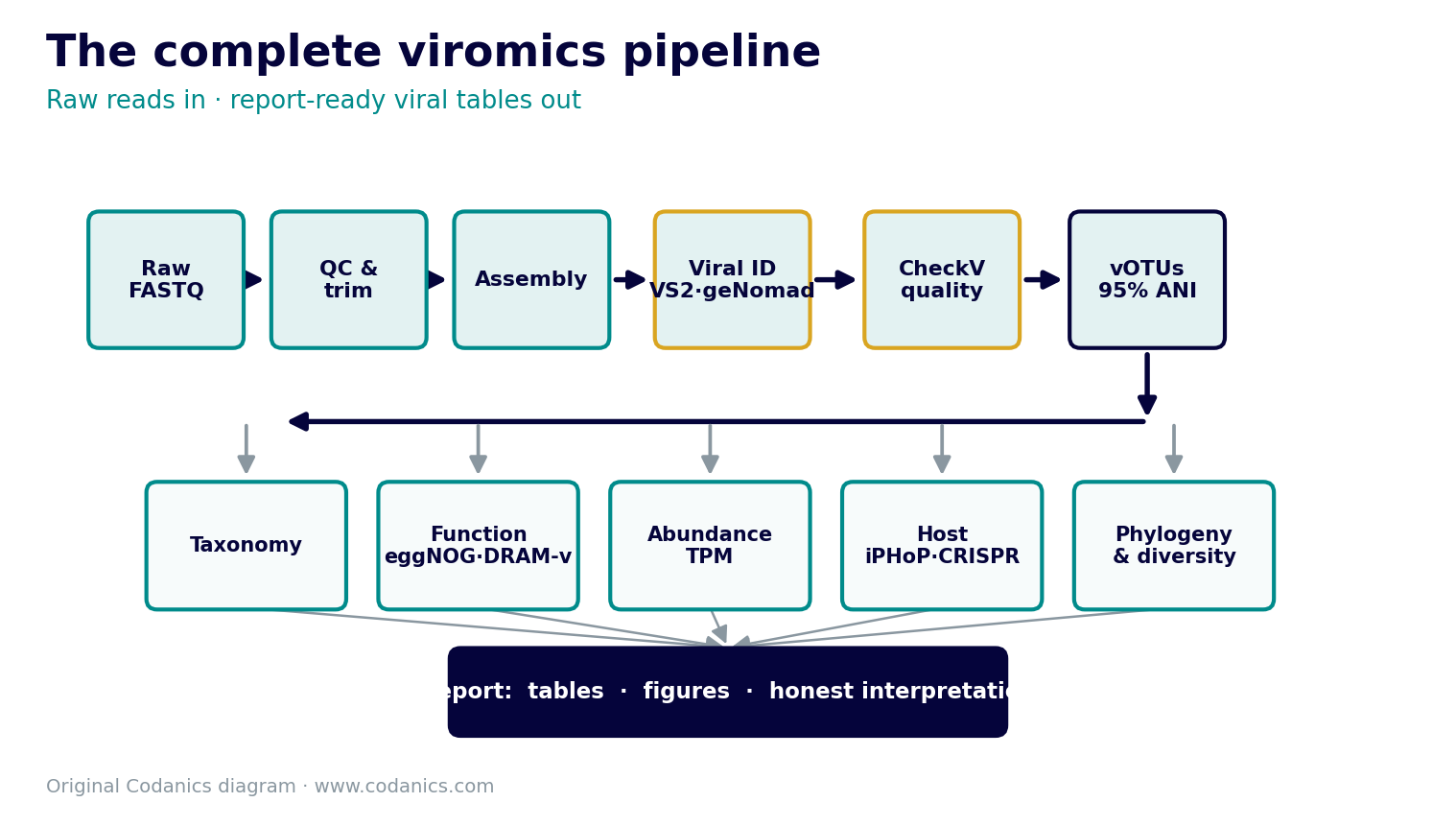{#fig-ch04 fig-alt="Complete viromics pipeline from raw reads to final report"}
::: {.callout-tip collapse="true"}
## 🎨 Generate this figure
**Save as:** `images/ch04-pipeline-overview.png` · **Aspect ratio:** 16:9 · **Style:** clean flat vector infographic, Codanics palette (teal `#008b8b`, navy `#05043b`, white background), no photorealism.
**Prompt:** Create a clean horizontal workflow infographic of a complete viromics analysis pipeline. From left to right, show labeled stages connected by arrows: paired-end FASTQ reads, quality control (FastQC/MultiQC), trimming (fastp), de novo assembly (MEGAHIT), assembly QC (QUAST), viral identification (VirSorter2 and geNomad), quality assessment (CheckV), and vOTU clustering. After vOTU clustering, fan the flow into five parallel downstream branches, each in its own rounded box: taxonomy, functional annotation, abundance mapping, host prediction, and phylogeny/diversity. Converge all branches into a final "report-ready tables" box on the right. Use small Linux-terminal icons on the compute steps, teal and navy Codanics branding, thin connecting arrows, and clear stage labels. No photorealism.
:::
## Quiz: Complete Pipeline
**Q1. Which step should happen before assembly?**
A. read QC and trimming
B. vConTACT2
C. host prediction
D. tree building
::: {.callout-note collapse='true'}
**Answer:** A. Low-quality reads and adapters should be handled before assembly.
:::
**Q2. What does CheckV estimate?**
A. viral quality and completeness
B. adapter sequence only
C. CPU temperature
D. sequencer model
::: {.callout-note collapse='true'}
**Answer:** A. CheckV is used for viral genome quality assessment.
:::
**Q3. What does mapping reads back to vOTUs estimate?**
A. abundance and coverage
B. Baltimore group
C. library kit price
D. host genome size
::: {.callout-note collapse='true'}
**Answer:** A. Coverage and TPM are calculated from mapped reads.
:::
**Q4. Why should taxonomy be conservative?**
A. many viruses are novel
B. all viruses are known
C. taxonomy is never needed
D. CheckV removes taxonomy
::: {.callout-note collapse='true'}
**Answer:** A. Reference databases are incomplete for viruses.
:::
**Q5. What is a good marker for viral phylogeny?**
A. one homologous viral gene family
B. all predicted proteins mixed together
C. FASTQ quality scores
D. adapter sequence
::: {.callout-note collapse='true'}
**Answer:** A. Phylogenies require homologous sequences.
:::
## Interactive quiz: Complete pipeline
```{=html}
<div class="interactive-quiz-note"><strong>How to use this quiz:</strong> Select one option, click <em>Check answer</em>, and read the explanation. Use the reset button if you want to try again.</div>
<div class="quiz-set">
<div class="quiz-question" data-answer="B">
<p class="quiz-prompt">1. Which tool in this pipeline is most directly associated with viral genome completeness assessment?</p>
<label class="quiz-option"><input type="radio" name="04-complete-pipeline-q1" value="A"> <strong>A.</strong> Bowtie2</label>
<label class="quiz-option"><input type="radio" name="04-complete-pipeline-q1" value="B"> <strong>B.</strong> CheckV</label>
<label class="quiz-option"><input type="radio" name="04-complete-pipeline-q1" value="C"> <strong>C.</strong> MAFFT</label>
<label class="quiz-option"><input type="radio" name="04-complete-pipeline-q1" value="D"> <strong>D.</strong> FastQC</label>
<div class="quiz-controls"><button type="button" class="quiz-check">Check answer</button><button type="button" class="quiz-reset">Reset</button></div>
<div class="quiz-explanation">CheckV estimates completeness, contamination, and quality tiers for metagenome-assembled viral genomes.</div>
<div class="quiz-feedback"></div>
</div>
<div class="quiz-question" data-answer="B">
<p class="quiz-prompt">2. Why map reads back to viral contigs after assembly?</p>
<label class="quiz-option"><input type="radio" name="04-complete-pipeline-q2" value="A"> <strong>A.</strong> To convert RNA to DNA</label>
<label class="quiz-option"><input type="radio" name="04-complete-pipeline-q2" value="B"> <strong>B.</strong> To estimate abundance and coverage</label>
<label class="quiz-option"><input type="radio" name="04-complete-pipeline-q2" value="C"> <strong>C.</strong> To remove all contamination</label>
<label class="quiz-option"><input type="radio" name="04-complete-pipeline-q2" value="D"> <strong>D.</strong> To skip taxonomy</label>
<div class="quiz-controls"><button type="button" class="quiz-check">Check answer</button><button type="button" class="quiz-reset">Reset</button></div>
<div class="quiz-explanation">Read mapping supports abundance estimation and helps confirm coverage across viral contigs or vOTUs.</div>
<div class="quiz-feedback"></div>
</div>
<div class="quiz-question" data-answer="B">
<p class="quiz-prompt">3. What does a vOTU represent in many viral ecology workflows?</p>
<label class="quiz-option"><input type="radio" name="04-complete-pipeline-q3" value="A"> <strong>A.</strong> A host chromosome</label>
<label class="quiz-option"><input type="radio" name="04-complete-pipeline-q3" value="B"> <strong>B.</strong> A viral operational taxonomic unit based on similarity thresholds</label>
<label class="quiz-option"><input type="radio" name="04-complete-pipeline-q3" value="C"> <strong>C.</strong> A sequencing lane</label>
<label class="quiz-option"><input type="radio" name="04-complete-pipeline-q3" value="D"> <strong>D.</strong> A protein family only</label>
<div class="quiz-controls"><button type="button" class="quiz-check">Check answer</button><button type="button" class="quiz-reset">Reset</button></div>
<div class="quiz-explanation">A vOTU is a practical grouping unit for viral sequences, commonly based on thresholds such as about 95 percent nucleotide identity.</div>
<div class="quiz-feedback"></div>
</div>
<div class="quiz-question" data-answer="B">
<p class="quiz-prompt">4. Which pair is best for a simple assembly-first viral discovery workflow?</p>
<label class="quiz-option"><input type="radio" name="04-complete-pipeline-q4" value="A"> <strong>A.</strong> FastQC and MultiQC only</label>
<label class="quiz-option"><input type="radio" name="04-complete-pipeline-q4" value="B"> <strong>B.</strong> VirSorter2 and CheckV</label>
<label class="quiz-option"><input type="radio" name="04-complete-pipeline-q4" value="C"> <strong>C.</strong> MAFFT and IQ-TREE only</label>
<label class="quiz-option"><input type="radio" name="04-complete-pipeline-q4" value="D"> <strong>D.</strong> ggplot2 and pheatmap</label>
<div class="quiz-controls"><button type="button" class="quiz-check">Check answer</button><button type="button" class="quiz-reset">Reset</button></div>
<div class="quiz-explanation">VirSorter2 predicts viral sequences and CheckV evaluates their quality, so together they form a strong core workflow.</div>
<div class="quiz-feedback"></div>
</div>
<div class="quiz-question" data-answer="B">
<p class="quiz-prompt">5. Why should taxonomy be interpreted conservatively?</p>
<label class="quiz-option"><input type="radio" name="04-complete-pipeline-q5" value="A"> <strong>A.</strong> Because all viruses are already cultured</label>
<label class="quiz-option"><input type="radio" name="04-complete-pipeline-q5" value="B"> <strong>B.</strong> Because many viral sequences are novel and reference databases are incomplete</label>
<label class="quiz-option"><input type="radio" name="04-complete-pipeline-q5" value="C"> <strong>C.</strong> Because taxonomy is irrelevant</label>
<label class="quiz-option"><input type="radio" name="04-complete-pipeline-q5" value="D"> <strong>D.</strong> Because geNomad always returns species names</label>
<div class="quiz-controls"><button type="button" class="quiz-check">Check answer</button><button type="button" class="quiz-reset">Reset</button></div>
<div class="quiz-explanation">Novelty is common in viromics. Family-level or higher-level assignments are often more reliable than overly specific labels.</div>
<div class="quiz-feedback"></div>
</div>
</div>
```
