8 End-to-End Mini Project
This chapter is the capstone: a complete, reproducible walkthrough that takes a real public sequencing run from the Sequence Read Archive all the way to a compact virome report. Nothing here is simulated. You will download the same bytes any other researcher would, mine viral contigs from a mixed wastewater metagenome, judge their quality honestly, cluster them into vOTUs, measure abundance, and write up what you can — and cannot — claim.
Think of it as the difference between practicing scales and playing a whole piece. Each previous chapter drilled one technique; here they connect into a single pipeline you can run end to end.
Learning objectives — by the end of this chapter you will be able to:
- retrieve and document a public SRA run with full provenance, using
prefetchandfasterq-dump; - run a quality-control, trimming, and assembly workflow on a real paired-end metagenome;
- mine viral contigs with two complementary tools (VirSorter2 and geNomad) and combine their candidates;
- use CheckV to filter recovered sequences to medium/high/complete quality with a safe fallback;
- dereplicate contigs into vOTUs, estimate abundance, and assemble a reproducible one-page report; and
- interpret metagenomic viral mining conservatively and avoid the most common analysis pitfalls.
This run is a shotgun wastewater metagenome: it contains bacterial, archaeal, and eukaryotic DNA alongside viral DNA, with no particle enrichment or capsid protection step. We are mining viral signal from a mixed community, not measuring a purified virome. That is exactly what makes it a good practice dataset — it forces you to separate real viral contigs from cellular background, which is the everyday reality of environmental viromics.
8.1 Run it all in one command
Once you understand each step below, the core pipeline — download through vOTU dereplication — is packaged in a single script. Download it, read it, then run it. (Annotation, abundance, figures, and the final report are then run as shown in the later steps.)
# After the databases and conda environments are in place:
bash run_mini_project_pipeline.sh    # or: bash ~/Downloads/run_mini_project_pipeline.sh
The rest of this chapter unpacks that script step by step so you understand every decision it makes.
8.2 Project title
Mining viral contigs from a public wastewater metagenome using Linux-based viral bioinformatics8.3 Research question
Can we recover putative viral contigs from a public paired-end wastewater metagenome,
assess their quality, cluster them into vOTUs, estimate abundance, and generate a
compact virome report?
8.4 Dataset provenance
Reproducibility starts with knowing exactly what you downloaded. The Sequence Read Archive stores raw sequencing data and supports reuse of public datasets (NCBI 2026). The full provenance for the run used here is:
| Field | Value |
|---|---|
| SRA run | SRR29680455 (NCBI Sequence Read Archive 2024) |
| BioProject | PRJNA527877 |
| Experiment | SRX25183710 |
| Sample | PHL1-P1-SS1 |
| Study name | PIRE: HEARD (Halting Environmental Antimicrobial Resistance Dissemination) |
| Sample type | wastewater secondary solids metagenome |
| Platform | Illumina NextSeq 500 |
| Layout | paired-end |
| Read length | 2 × 75 bp |
| Download size | ~458.7 MB |
| Spots | 7,366,184 |
| Published | July 2, 2024 |
The parent project surveys metagenomes from municipal wastewater treatment plants; the selected experiment used shotgun metagenomic sequencing with Illumina NextSeq 500 2 × 75 bp paired-end reads (NCBI Sequence Read Archive 2024). prefetch and fasterq-dump are the standard SRA Toolkit commands for downloading and converting public runs (NCBI Sequence Read Archive 2022).
8.5 Expected final outputs
1. Raw FASTQ files from SRA          6. CheckV quality table
2. QC reports                        7. vOTU representative FASTA
3. Trimmed reads                     8. Viral abundance table
4. Metagenomic assembly              9. Basic taxonomy / annotation outputs
5. Putative viral contigs           10. Final mini virome report
8.6 Step 1: Create the project folder
mkdir -p ~/viromics_course/mini_project_wastewater
cd ~/viromics_course/mini_project_wastewater

mkdir -p raw_reads trimmed_reads qc_reports assemblies assembly_qc \
  viral_identification checkv votus taxonomy annotation abundance \
  visualization reports logs scripts databases
Set the environment variables the whole pipeline reuses. Defining them once, up front, keeps every later command short and consistent.
export PROJECT=$HOME/viromics_course/mini_project_wastewater
export THREADS=12
export SRA_ID=SRR29680455
export SAMPLE=samples

# Database locations (define before first use)
export VIROME_DB=$HOME/viromics_course/databases
export CHECKVDB=$VIROME_DB/checkv-db
export EGGNOG_DATA_DIR=$VIROME_DB/eggnog

cd $PROJECT
8.7 Step 2: Record the metadata
A metadata file travels with your results and makes them reproducible.
cat > metadata.tsv << 'EOF'
sample_id   sra_run bioproject  experiment  sample  environment sample_type platform    layout  read_length strategy
samples SRR29680455 PRJNA527877 SRX25183710 PHL1-P1-SS1 wastewater  secondary_solids    Illumina_NextSeq_500    paired  2x75    WGS_metagenome
EOF

column -t -s $'\t' metadata.tsv
8.8 Step 3: Download and convert the SRA run
conda activate viromics-core

prefetch $SRA_ID --output-directory raw_reads

fasterq-dump \
  raw_reads/$SRA_ID \
  --split-files \
  --threads $THREADS \
  --outdir raw_reads

pigz -p $THREADS raw_reads/${SRA_ID}_1.fastq
pigz -p $THREADS raw_reads/${SRA_ID}_2.fastq

# Give the files the simple sample names used throughout
ln -sf ${PROJECT}/raw_reads/${SRA_ID}_1.fastq.gz raw_reads/samples_R1.fastq.gz
ln -sf ${PROJECT}/raw_reads/${SRA_ID}_2.fastq.gz raw_reads/samples_R2.fastq.gz

seqkit stats raw_reads/samples_R1.fastq.gz raw_reads/samples_R2.fastq.gz
seqkit gives fast summary statistics for FASTA/FASTQ files (Shen et al. 2016).
Estimated resources on 12 threads and 32 GB RAM: download and conversion usually take 20 to 60 minutes depending on internet and disk speed. Keep 10 to 20 GB free because fasterq-dump writes temporary files before compression.
8.9 Step 4: QC and trimming
Inspect the raw reads first, then trim adapters and low-quality tails.
mkdir -p qc_reports/fastqc_raw qc_reports/multiqc_raw

fastqc -t $THREADS -o qc_reports/fastqc_raw \
  raw_reads/samples_R1.fastq.gz raw_reads/samples_R2.fastq.gz

multiqc qc_reports/fastqc_raw \
  -o qc_reports/multiqc_raw \
  -n samples_raw_multiqc.html
mkdir -p trimmed_reads qc_reports/fastp logs
fastp \
-i raw_reads/samples_R1.fastq.gz \
-I raw_reads/samples_R2.fastq.gz \
-o trimmed_reads/samples_R1.fastp.fastq.gz \
-O trimmed_reads/samples_R2.fastp.fastq.gz \
--detect_adapter_for_pe \
--cut_front \
--cut_tail \
--cut_window_size 4 \
--cut_mean_quality 20 \
--length_required 50 \
--thread $THREADS \
--html qc_reports/fastp/samples_fastp.html \
--json qc_reports/fastp/samples_fastp.json \
> logs/samples_fastp.log 2>&1
seqkit stats \
raw_reads/samples_R1.fastq.gz raw_reads/samples_R2.fastq.gz \
trimmed_reads/samples_R1.fastp.fastq.gz trimmed_reads/samples_R2.fastp.fastq.gzEstimated resources on 12 threads and 32 GB RAM: 15 to 45 minutes. Storage after trimming can reach several GB.
8.10 Step 5: Assembly and assembly QC
MEGAHIT is fast and memory-light, which makes it a good first choice for a first assembly.
mkdir -p assemblies logs

megahit \
  -1 trimmed_reads/samples_R1.fastp.fastq.gz \
  -2 trimmed_reads/samples_R2.fastp.fastq.gz \
  -o assemblies/megahit_samples \
  --min-contig-len 1000 \
  -t $THREADS \
  > logs/samples_megahit.log 2>&1

export CONTIGS=$PROJECT/assemblies/megahit_samples/final.contigs.fa
seqkit stats $CONTIGS
grep -c "^>" $CONTIGS
mkdir -p assembly_qc/quast_megahit
quast.py \
$CONTIGS \
-o assembly_qc/quast_megahit \
-t $THREADS \
--min-contig 1000QUAST reports contig counts, N50, and total assembly length (Gurevich et al. 2013).
Estimated resources on 12 threads and 32 GB RAM: MEGAHIT may take 30 minutes to 3 hours. Keep 30 to 80 GB free for temporary assembly files.
8.15 Step 10: Filter to medium/high/complete quality
Never trust column positions from memory — CheckV’s layout can change between versions. Always inspect the header first.
head -n 1 checkv/checkv_samples/quality_summary.tsv | tr '\t' '\n' | nlIn current CheckV, the quality label lives in column 8. Extract the IDs of contigs judged Medium-quality or better:
awk -F'\t' '
NR==1 {next}
$8=="Medium-quality" || $8=="High-quality" || $8=="Complete" {
  print $1
}' checkv/checkv_samples/quality_summary.tsv \
> checkv/checkv_samples/samples_medium_high_complete_ids.txt

seqkit grep \
  -f checkv/checkv_samples/samples_medium_high_complete_ids.txt \
  checkv/checkv_samples/samples_checkv_combined_viral.fna \
  > checkv/checkv_samples/samples_medium_high_complete_viral.fna

seqkit stats checkv/checkv_samples/samples_medium_high_complete_viral.fna
A shotgun metagenome may recover no medium-or-better viral genomes, which would leave the filtered file empty and break every downstream step. Guard against that with a simple fallback — if the filtered file is non-empty use it, otherwise keep all CheckV viral contigs:
if [ -s checkv/checkv_samples/samples_medium_high_complete_viral.fna ]; then
  export VIRAL_FASTA=$PROJECT/checkv/checkv_samples/samples_medium_high_complete_viral.fna
else
  export VIRAL_FASTA=$PROJECT/checkv/checkv_samples/samples_checkv_combined_viral.fna
fi
echo "Using viral FASTA: $VIRAL_FASTA"
8.16 Step 11: Dereplicate into vOTUs
Cluster near-identical contigs into viral operational taxonomic units (vOTUs) at 95% nucleotide identity over 85% of the shorter sequence — the community-standard (MIUViG) species-level threshold (Roux et al. 2019).
conda activate viromics-core
cd $PROJECT

mkdir -p votus/cdhit_samples

cd-hit-est \
  -i $VIRAL_FASTA \
  -o votus/cdhit_samples/samples_votus_95.fa \
  -c 0.95 \
  -aS 0.85 \
  -G 0 \
  -g 1 \
  -T $THREADS \
  -M 0

export VOTU_FASTA=$PROJECT/votus/cdhit_samples/samples_votus_95.fa
seqkit stats $VOTU_FASTA
Estimated resources on 12 threads and 32 GB RAM: usually minutes for this mini project. Storage under 5 GB.
8.17 Step 12: Gene prediction and functional annotation
Predict genes on the vOTU representatives with Prodigal (Hyatt et al. 2010), then annotate with eggNOG-mapper.
mkdir -p annotation/prodigal

prodigal \
  -i $VOTU_FASTA \
  -a annotation/prodigal/samples_votus.faa \
  -d annotation/prodigal/samples_votus.genes.fna \
  -o annotation/prodigal/samples_votus.gff \
  -f gff \
  -p meta

seqkit stats annotation/prodigal/samples_votus.faa
conda activate eggnog
cd $PROJECT
mkdir -p annotation/eggnog logs
emapper.py \
-i annotation/prodigal/samples_votus.faa \
--itype proteins \
-m diamond \
--cpu $THREADS \
--data_dir $EGGNOG_DATA_DIR \
-o samples_eggnog \
--output_dir annotation/eggnog \
> logs/samples_eggnog.log 2>&1
grep -v "^#" annotation/eggnog/samples_eggnog.emapper.annotations | headEstimated resources on 12 threads and 32 GB RAM: Prodigal takes seconds to minutes. eggNOG can take minutes to hours depending on protein count and database storage speed.
8.18 Step 13: Abundance mapping
Map trimmed reads back to the vOTUs with Bowtie2 (Langmead and Salzberg 2012), sort with samtools (Danecek et al. 2021), then compute coverage and TPM with CoverM.
conda activate viromics-core
cd $PROJECT

mkdir -p abundance/bowtie2_index abundance/logs

bowtie2-build $VOTU_FASTA abundance/bowtie2_index/samples_votus

bowtie2 \
  -x abundance/bowtie2_index/samples_votus \
  -1 trimmed_reads/samples_R1.fastp.fastq.gz \
  -2 trimmed_reads/samples_R2.fastp.fastq.gz \
  -p $THREADS \
  --very-sensitive \
  2> abundance/logs/samples_bowtie2_mapping.log \
| samtools view -bS - \
| samtools sort -@ $THREADS -o abundance/samples_vs_votus.sorted.bam

samtools index abundance/samples_vs_votus.sorted.bam
samtools flagstat abundance/samples_vs_votus.sorted.bam > abundance/samples_flagstat.txt

coverm contig \
  --bam-files abundance/samples_vs_votus.sorted.bam \
  --methods mean covered_fraction count tpm \
  --threads $THREADS \
  > abundance/samples_coverm_contig.tsv
Estimated resources on 12 threads and 32 GB RAM: 15 minutes to 2 hours. BAM files can require several GB.
8.19 Step 14: Report tables
Again, inspect the CheckV header before slicing columns, then build clean, minimal tables for reporting.
mkdir -p reports/tables visualization/figures

head -n 1 checkv/checkv_samples/quality_summary.tsv | tr '\t' '\n' | nl

awk -F'\t' '
BEGIN{OFS="\t"}
NR==1 {print "contig_id","length","completeness","quality"}
NR>1  {print $1,$2,$10,$8}
' checkv/checkv_samples/quality_summary.tsv \
> reports/tables/checkv_quality_clean.tsv

seqkit fx2tab -n -l $VOTU_FASTA > reports/tables/votu_lengths.tsv
cp abundance/samples_coverm_contig.tsv reports/tables/votu_abundance_coverm.tsv
8.20 Step 15: Figures
The two figures below are illustrative example outputs, generated by scripts/make_figures.py from the example tables in data/example/. On your own run, the exact bars and lengths will depend on how much viral signal this dataset yields on your machine. The short R snippet that follows shows how to build the same two figures from your Step 14 report tables.
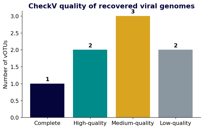
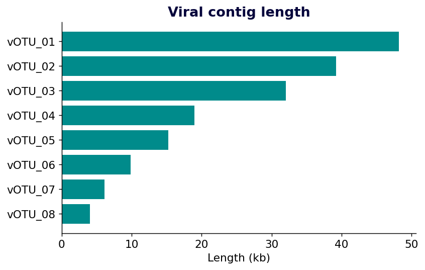
This mini-project snippet reads your Step 14 report tables and writes both figures into visualization/figures:
library(readr); library(dplyr); library(ggplot2)

# Figure 1: CheckV quality categories
checkv <- read_tsv("reports/tables/checkv_quality_clean.tsv", show_col_types = FALSE)
ggplot(count(checkv, quality), aes(quality, n)) +
  geom_col(width = 0.7) +
  labs(title = "CheckV quality of recovered vOTUs",
       x = "Quality category", y = "Number of viral contigs") +
  theme_bw(base_size = 12)
ggsave("visualization/figures/fig-checkv-quality.png", width = 6, height = 4, dpi = 300)

# Figure 2: viral contig length distribution
lengths <- read_tsv("reports/tables/votu_lengths.tsv",
                    col_names = c("votu_id", "length"), show_col_types = FALSE)
ggplot(lengths, aes(length / 1000)) +
  geom_histogram(bins = 20) +
  labs(title = "Viral contig lengths", x = "Length (kb)", y = "Number of vOTUs") +
  theme_bw(base_size = 12)
ggsave("visualization/figures/fig-contig-length.png", width = 6, height = 4, dpi = 300)# Regenerate the illustrative example figures shown above
python scripts/make_figures.py
# ...or save the snippet above as a script and run it on your own tables
ls -lh visualization/figures/8.21 Step 16: Final report
The reporting script gathers the key statistics and file paths into a single plain-text summary you can hand in with your deliverables.
bash scripts/create_report_summary.sh "$PROJECT" "$SAMPLE"
cat reports/${SAMPLE}_viromics_summary.txt
The script records raw, trimmed, assembly, viral, and vOTU statistics; the paths of every important output (MultiQC, fastp, QUAST, VirSorter2, geNomad, CheckV, vOTU FASTA, abundance table, figures); and a short interpretation guide reminding the reader that this is a shotgun metagenome and that predictions are putative.
8.22 How to interpret your results
Use these points when explaining — and grading — the project:
- This is metagenomic viral mining, not a pure virome experiment. The library contains bacteria, archaea, eukaryotic DNA, and viral DNA all mixed together. Every viral contig has to be pulled out of that background, so “how much virus did we find” is really “how much viral signal survived identification and quality filtering.”
- VirSorter2 and geNomad predict candidates; they do not confirm viruses. Each is a probabilistic classifier. Combining them raises sensitivity, but a call from either tool is still a hypothesis.
- CheckV is essential. Many recovered contigs are incomplete fragments or carry host flanks. Reporting a fragment as if it were a finished genome is the fastest way to overstate a result. Completeness and contamination estimates are what make the recovered set defensible.
- A vOTU is a clustered viral unit, not a named species. Dereplicating at ~95% nucleotide identity gives an operational, species-level grouping. It says “these contigs represent the same viral population,” not “this is Escherichia phage X.”
- Coverage and TPM measure abundance; assembly only measures recovery. A contig existing tells you it assembled well; its TPM tells you how common those reads were. Do not confuse “we assembled it” with “it was abundant.”
- Taxonomy and host prediction must stay conservative — especially for wastewater. Wastewater pools human, animal, plant, and environmental sources, so a computational host or taxonomy call is a candidate association, not a confirmed one. Prefer family-level (or higher) labels for novel contigs.
- Report the protocol, not just the numbers. Because a virome is protocol-dependent, your write-up should state that this is a shotgun (non-enriched) metagenome so readers can calibrate what “we recovered N vOTUs” actually means.
- Skipping the CheckV filter and reporting every VirSorter2/geNomad hit as a “virus.”
- Hard-coding CheckV column numbers instead of checking the header with
head -n1 ... | tr '\t' '\n' | nl— the layout shifts between versions. - Letting an empty medium/high/complete file crash the pipeline because you forgot the fallback
export VIRAL_FASTAbranch. - Claiming confirmed hosts or species from computational predictions on a mixed wastewater sample.
- Confusing assembly recovery with abundance — a long contig is not necessarily a common one.
- Reporting raw read counts as “the virome” without noting this is a non-enriched shotgun metagenome.
8.23 Project deliverables
A complete project should produce:
1. raw MultiQC report
2. trimmed fastp HTML report
3. QUAST assembly report
4. VirSorter2 viral score table (and geNomad summary if produced)
5. CheckV quality_summary.tsv
6. vOTU FASTA file
7. CoverM abundance table
8. two figures:
   - CheckV quality bar plot
   - viral contig length distribution
9. one-page interpretation report
Suggested report title:
Viral contig recovery and quality assessment from a public wastewater metagenome8.24 Key takeaways
- Reproducibility starts with provenance: document the exact SRA run (here
SRR29680455, BioProject PRJNA527877) and every tool and parameter before reporting a single result (NCBI Sequence Read Archive 2024). - This is shotgun viral mining, not a purified virome — viral contigs must be separated from bacterial, archaeal, and eukaryotic background, so “how much virus we found” means “how much viral signal survived identification and quality filtering”.
- Two complementary identifiers raise sensitivity: VirSorter2 and geNomad use different models, and their pooled candidates outperform either alone (Guo et al. 2021; Camargo et al. 2024).
- CheckV is the key quality gate — completeness and contamination estimates decide which contigs are defensible, and a fallback branch prevents an empty medium/high/complete file from crashing downstream steps (Nayfach et al. 2021).
- A vOTU is a clustered, species-level viral population (~95% ANI), not a named species; coverage and TPM measure abundance, while assembly only measures recovery.
- Keep taxonomy and host predictions conservative, especially for pooled wastewater sources, and always inspect a table header before slicing columns by position.
8.25 Further reading
- The SRA run record and its metadata for the wastewater dataset used throughout this chapter (NCBI Sequence Read Archive 2024).
- Overview of the Sequence Read Archive and how public runs are retrieved and reused (NCBI 2026).
- CheckV for viral genome quality assessment (Nayfach et al. 2021) and MEGAHIT for the metagenomic assembly step (Li et al. 2015).
- NCBI SRA Toolkit documentation for
prefetchandfasterq-dump— https://github.com/ncbi/sra-tools.
8.26 Chapter figure
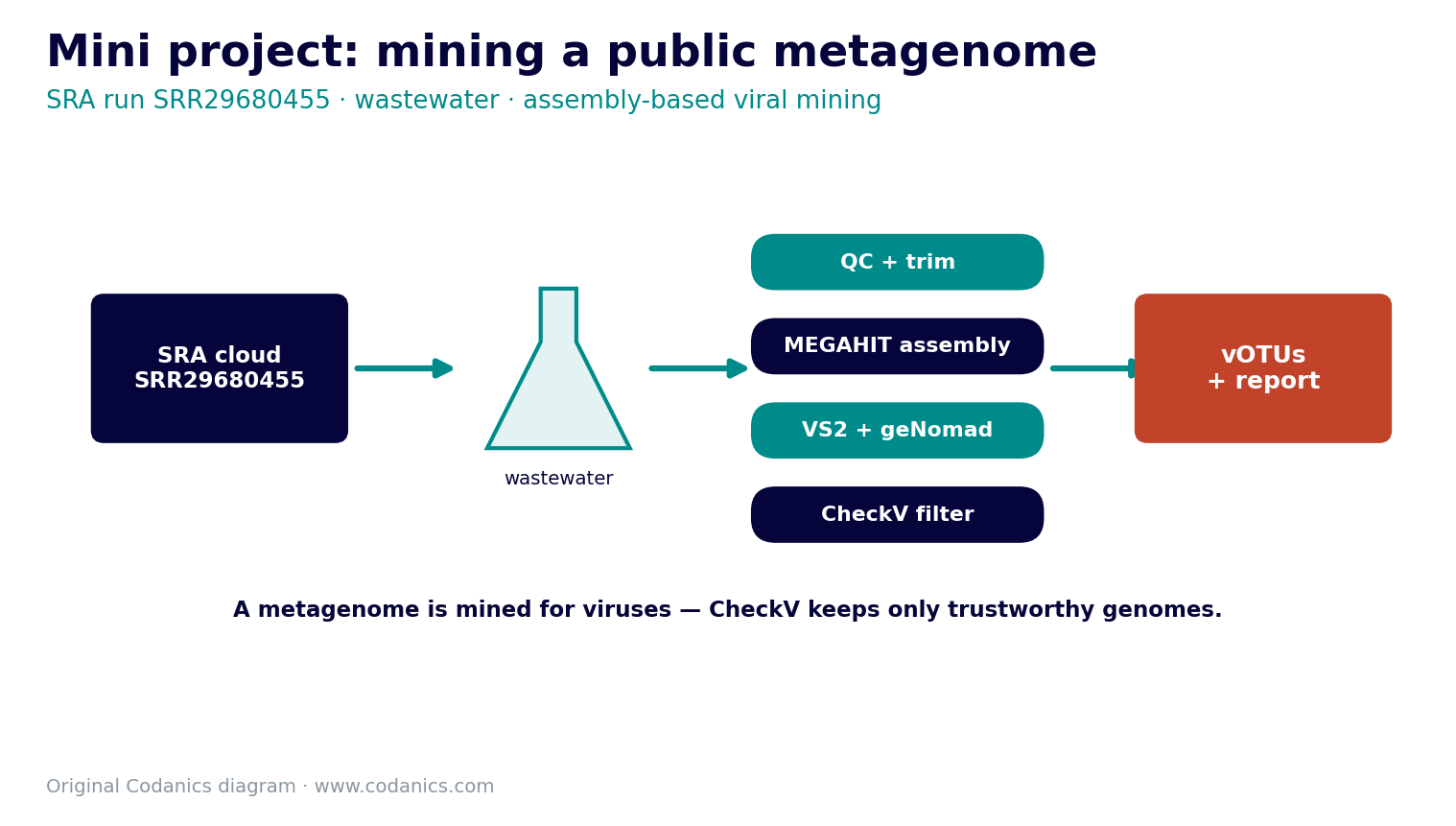
Save as: images/ch06-wastewater-miniproject.png · Aspect ratio: 16:9 · Style: clean flat vector infographic, Codanics palette (teal #008b8b, navy #05043b, white background), no photorealism.
Prompt: Create a clean educational workflow infographic for a wastewater viral-mining mini project, laid out left to right as a horizontal pipeline of connected labeled stages. Start with a small wastewater-treatment icon and a database cylinder labeled “Public SRA run SRR29680455”, then arrows through boxes labeled in order: “Download (prefetch / fasterq-dump)”, “QC and trimming (FastQC, fastp)”, “Assembly (MEGAHIT)”, “Viral identification (VirSorter2 + geNomad)” shown as two parallel boxes merging into “Combined candidates”, “Quality control (CheckV)”, “vOTU clustering (95% ANI, CD-HIT-EST)”, “Abundance (Bowtie2 + CoverM)”, and ending in a document icon labeled “Virome report + figures”. Use teal and navy Codanics branding, rounded boxes, clear arrows, and small monochrome icons for each stage. No photorealism, white background, readable sans-serif labels.
8.27 Quiz: Mini Project
Q1. What is the SRA run used in this mini project?
A. SRR29680455 B. SRR000001 C. ERR123456 D. SAMN00000
Answer: A. The selected public run is SRR29680455 (BioProject PRJNA527877, experiment SRX25183710, sample PHL1-P1-SS1).
Q2. Why is this dataset described as viral mining?
A. it is a shotgun metagenome, not virus-enriched B. it contains only pure viral particles C. it has no bacterial reads D. it is a PCR assay
Answer: A. Viral contigs are mined from mixed metagenomic reads that also contain cellular DNA.
Q3. Which command converts SRA data to FASTQ?
A. fasterq-dump B. fastqc C. quast.py D. iqtree
Answer: A. fasterq-dump converts prefetched SRA data to FASTQ.
Q4. Why does the pipeline run both VirSorter2 and geNomad?
A. they use different models and recover complementary candidates B. one converts FASTQ and the other assembles C. geNomad replaces CheckV D. only to double the runtime
Answer: A. No single identifier catches every virus, so their candidates are combined before quality control.
Q5. What should the CheckV step guard against when filtering to medium/high/complete?
A. an empty filtered file breaking downstream steps B. too many complete genomes C. missing raw reads D. adapter contamination
Answer: A. A shotgun metagenome may yield no medium-or-better genomes, so a fallback export VIRAL_FASTA keeps the pipeline running on all CheckV viral contigs.
8.28 Interactive quiz: Mini project
1. Which public run is used in the mini project?
2. What is the sample type in the mini project?
3. Why is this project a good practice example?
4. Which tools are used to download and convert the public run?
5. Which output is most important for judging viral genome quality in the mini project?