Category: machine learning

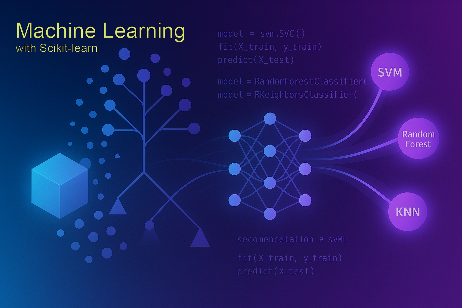
Scikit-Learn Mastery Guide: Complete Machine Learning in Python | ML Engineer Blog 0% 🌙 ↑ Scikit-Learn Mastery Guide: Complete Machine Learning in Python 🤖 Scikit-learn is the most popular and comprehensive machine learning library in Python, providing simple and efficient tools for data mining and data analysis. Whether you're a beginner taking your first steps into machine learning or an experienced practitioner looking to implement production-ready models, this guide will take you from basic concepts to advanced techniques. In this comprehensive ML engineering guide, we'll explore every major algorithm in scikit-learn with practical examples using built-in datasets, demonstrating real-world applications and best practices for modern machine learning workflows. Master Machine Learning with Python's Most Trusted Library 🎥 Machine Learning in Python: Complete Crash Course (2-Part Series) Machine Learning in Python | Complete Crash Course | Python | Scikit-learn | (Part-1/2) Machine Learning in Python | Complete Crash Course | Python | Scikit-learn | (Part-2/2) These two lectures provide a complete, hands-on introduction to machine learning in Python using scikit-learn. Watch both parts to master the fundamentals and practical workflow of ML in Python! Table of Contents Why Scikit-Learn is Essential for ML Installation with Conda Environment Benefits of Using Scikit-Learn ML Basics and Core Concepts Supervised Learning Algorithms Unsupervised Learning Algorithms Model Selection and Evaluation Data Preprocessing and Feature Engineering ML Pipelines and Automation Best Practices and Performance Tips Real-World Applications Conclusion Why Scikit-Learn is Essential for ML Engineers Industry Standard: Used by data scientists Professionals who extract insights from data using statistical methods, machine learning, and domain expertise. , ML engineers, and researchers worldwide Comprehensive Library: Covers supervised, unsupervised, and semi-supervised learning Production Ready: Optimized for performance with robust, well-tested implementations Consistent API: All estimators follow the same interface pattern (fit, predict, transform) Excellent Documentation: Comprehensive examples and theoretical background Active Community: Continuous development with regular releases and improvements Integration Friendly: Works seamlessly with NumPy Fundamental package for scientific computing with Python. , Pandas Data manipulation and analysis library for Python. , and visualization libraries Installation with Conda Environment Setting up a proper environment is crucial for ML projects. Here's how to install scikit-learn using conda: Step 1: Create a New Conda Environment # Create a new environment named 'ml-env' with Python 3.9 conda create -n ml-env python=3.9 # Activate the environment conda activate ml-env Step 2: Install Scikit-Learn and Dependencies # Install scikit-learn and essential data science packages conda install scikit-learn pandas numpy matplotlib seaborn jupyter # Alternative: Install from conda-forge (recommended for latest versions) conda install -c conda-forge scikit-learn pandas numpy matplotlib seaborn # Install additional ML libraries conda install -c conda-forge xgboost lightgbm plotly Step 3: Verify Installation import sklearn import pandas as pd import numpy as np import matplotlib.pyplot as plt print(f"Scikit-learn version: {sklearn.__version__}") print(f"NumPy version: {np.__version__}") print(f"Pandas version: {pd.__version__}") # Test with a simple example from sklearn.datasets import load_iris from sklearn.model_selection import train_test_split from sklearn.ensemble import RandomForestClassifier # Load sample data iris = load_iris() X_train, X_test, y_train, y_test = train_test_split( iris.data, iris.target, test_size=0.3, random_state=42 ) # Create and train model model = RandomForestClassifier(random_state=42) model.fit(X_train, y_train) accuracy = model.score(X_test, y_test) print(f"Installation successful! Test accuracy: {accuracy:.2f}") Managing Dependencies # Export environment for reproducibility conda env export > ml-environment.yml # Create environment from file conda env create -f ml-environment.yml # List installed packages conda list # Update scikit-learn conda update scikit-learn Benefits of Using Scikit-Learn 🚀 Ease of Use Consistent API across all algorithms makes learning and switching between models seamless. The fit/predict pattern is intuitive and reduces cognitive overhead. ⚡ Performance Optimized implementations in C/Cython provide excellent performance. Many algorithms support parallel processing and are memory-efficient. 🔧 Complete Toolkit Everything you need for ML workflows: preprocessing, feature selection, model training, evaluation, and hyperparameter tuning in one package. 📊 Built-in Datasets Comes with classic datasets for learning and benchmarking, making it easy to start experimenting immediately. 🏭 Production Ready Battle-tested in production environments with robust error handling, extensive testing, and stable APIs. ML Basics and Core Concepts Understanding the Scikit-Learn API import numpy as np import pandas as pd from sklearn.datasets import load_iris, load_boston, load_wine from sklearn.model_selection import train_test_split from sklearn.preprocessing import StandardScaler from sklearn.metrics import accuracy_score, mean_squared_error # Load a sample dataset iris = load_iris() print("Dataset shape:", iris.data.shape) print("Feature names:", iris.feature_names) print("Target names:", iris.target_names) # The standard ML workflow X, y = iris.data, iris.target # 1. Split the data X_train, X_test, y_train, y_test = train_test_split( X, y, test_size=0.2, random_state=42, stratify=y ) # 2. Preprocess (optional) scaler = StandardScaler() X_train_scaled = scaler.fit_transform(X_train) X_test_scaled = scaler.transform(X_test) print(f"Training set shape: {X_train.shape}") print(f"Test set shape: {X_test.shape}") print(f"Class distribution: {np.bincount(y_train)}") Essential ML Concepts # Supervised vs Unsupervised Learning Examples from sklearn.cluster import KMeans from sklearn.decomposition import PCA # Supervised Learning - we have target labels from sklearn.svm import SVC supervised_model = SVC() supervised_model.fit(X_train, y_train) predictions = supervised_model.predict(X_test) print(f"Supervised accuracy: {accuracy_score(y_test, predictions):.3f}") # Unsupervised Learning - no target labels unsupervised_model = KMeans(n_clusters=3, random_state=42) clusters = unsupervised_model.fit_predict(X) print(f"Cluster centers shape: {unsupervised_model.cluster_centers_.shape}") # Dimensionality Reduction pca = PCA(n_components=2) X_reduced = pca.fit_transform(X) print(f"Explained variance ratio: {pca.explained_variance_ratio_}") print(f"Reduced data shape: {X_reduced.shape}") Supervised Learning Algorithms Supervised learning uses labeled data to learn a mapping from inputs to outputs. Let's explore each major algorithm with practical examples. 1. Linear Regression Linear Regression - Predicting Continuous Values Best for: Predicting continuous numerical values with linear relationships # Linear Regression Example with Boston Housing Dataset from sklearn.datasets import fetch_california_housing from sklearn.linear_model import LinearRegression from sklearn.metrics import mean_squared_error, r2_score import matplotlib.pyplot as plt # Load California housing dataset (Boston dataset is deprecated) housing = fetch_california_housing() X, y = housing.data, housing.target # Use only a few features for simplicity feature_names = housing.feature_names X_simple = X[:, [0, 5, 6]] # MedInc, AveRooms, AveBedrms feature_names_simple = [feature_names[i] for i in [0, 5, 6]] # Split the data X_train, X_test, y_train, y_test = train_test_split( X_simple, y, test_size=0.2, random_state=42 ) # Create and train the model lr_model = LinearRegression() lr_model.fit(X_train, y_train) # Make predictions y_pred = lr_model.predict(X_test) # Evaluate the model mse = mean_squared_error(y_test, y_pred) r2 = r2_score(y_test, y_pred) print("Linear Regression Results:") print(f"Mean Squared Error: {mse:.3f}") print(f"R² Score: {r2:.3f}") print(f"Coefficients: {lr_model.coef_}") print(f"Intercept: {lr_model.intercept_:.3f}") # Feature importance for feature, coef in zip(feature_names_simple, lr_model.coef_): print(f"{feature}: {coef:.3f}") 2. Logistic Regression Logistic Regression - Binary and Multi-class Classification Best for: Classification problems with interpretable results and probability estimates # Logistic Regression with Wine Dataset from sklearn.datasets import load_wine from sklearn.linear_model import LogisticRegression from sklearn.metrics import classification_report, confusion_matrix import seaborn as sns # Load wine dataset wine = load_wine() X, y = wine.data, wine.target # Split the data X_train, X_test, y_train, y_test = train_test_split( X, y, test_size=0.2, random_state=42, stratify=y ) # Scale the features (important for logistic regression) scaler = StandardScaler() X_train_scaled = scaler.fit_transform(X_train) X_test_scaled = scaler.transform(X_test) # Create and train the model log_reg = LogisticRegression(random_state=42, max_iter=1000) log_reg.fit(X_train_scaled, y_train) # Make predictions y_pred = log_reg.predict(X_test_scaled) y_pred_proba = log_reg.predict_proba(X_test_scaled) # Evaluate the model accuracy = accuracy_score(y_test, y_pred) print("Logistic Regression Results:") print(f"Accuracy: {accuracy:.3f}") print("\nClassification Report:") print(classification_report(y_test, y_pred, target_names=wine.target_names)) # Confusion Matrix cm = confusion_matrix(y_test, y_pred) print(f"\nConfusion Matrix:\n{cm}") # Feature importance (coefficients) feature_importance = pd.DataFrame({ 'feature': wine.feature_names, 'importance': np.abs(log_reg.coef_[0]) # Taking first class coefficients }).sort_values('importance', ascending=False) print("\nTop 5 Most Important Features:") print(feature_importance.head()) 3. Decision Trees Decision Trees - Interpretable Non-linear Models Best for: Problems requiring interpretability and handling non-linear relationships # Decision Tree with Iris Dataset from sklearn.datasets import load_iris from sklearn.tree import DecisionTreeClassifier, plot_tree from sklearn.metrics import accuracy_score # Load iris dataset iris = load_iris() X, y = iris.data, iris.target # Split the data X_train, X_test, y_train, y_test = train_test_split( X, y, test_size=0.2, random_state=42, stratify=y ) # Create and train the model dt_model = DecisionTreeClassifier( max_depth=3, # Limit depth to prevent overfitting min_samples_split=5, min_samples_leaf=2, random_state=42 ) dt_model.fit(X_train, y_train) # Make predictions y_pred = dt_model.predict(X_test) # Evaluate the model accuracy = accuracy_score(y_test, y_pred) print("Decision Tree Results:") print(f"Accuracy: {accuracy:.3f}") # Feature importance feature_importance = pd.DataFrame({ 'feature': iris.feature_names, 'importance': dt_model.feature_importances_ }).sort_values('importance', ascending=False) print("\nFeature Importance:") print(feature_importance) # Tree depth and leaves info print(f"\nTree depth: {dt_model.get_depth()}") print(f"Number of leaves: {dt_model.get_n_leaves()}") # You can visualize the tree (uncomment to see) # plt.figure(figsize=(15, 10)) # plot_tree(dt_model, feature_names=iris.feature_names, # class_names=iris.target_names, filled=True, rounded=True) # plt.show() 4. Random Forest Random Forest - Ensemble of Decision Trees Best for: High accuracy with built-in feature importance and reduced overfitting # Random Forest with Breast Cancer Dataset from sklearn.datasets import load_breast_cancer from sklearn.ensemble import RandomForestClassifier from sklearn.metrics import accuracy_score, roc_auc_score # Load breast cancer dataset cancer = load_breast_cancer() X, y = cancer.data, cancer.target # Split the data X_train, X_test, y_train, y_test = train_test_split( X, y, test_size=0.2, random_state=42, stratify=y ) # Create and train the model rf_model = RandomForestClassifier( n_estimators=100, # Number of trees max_depth=10, min_samples_split=5, min_samples_leaf=2, random_state=42, n_jobs=-1 # Use all available cores ) rf_model.fit(X_train, y_train) # Make predictions y_pred = rf_model.predict(X_test) y_pred_proba = rf_model.predict_proba(X_test)[:, 1] # Probability of positive class # Evaluate the model accuracy = accuracy_score(y_test, y_pred) auc_score = roc_auc_score(y_test, y_pred_proba) print("Random Forest Results:") print(f"Accuracy: {accuracy:.3f}") print(f"AUC Score: {auc_score:.3f}") # Feature importance feature_importance = pd.DataFrame({ 'feature': cancer.feature_names, 'importance': rf_model.feature_importances_ }).sort_values('importance', ascending=False) print("\nTop 10 Most Important Features:") print(feature_importance.head(10)) # Out-of-bag score (built-in cross-validation) rf_oob = RandomForestClassifier( n_estimators=100, oob_score=True, random_state=42 ) rf_oob.fit(X_train, y_train) print(f"\nOut-of-bag score: {rf_oob.oob_score_:.3f}") 5. Support Vector Machine (SVM) Support Vector Machine - Maximum Margin Classifier Best for: High-dimensional data, text classification, and when you need robust performance # SVM with Digits Dataset from sklearn.datasets import load_digits from sklearn.svm import SVC from sklearn.metrics import accuracy_score, classification_report # Load digits dataset digits = load_digits() X, y = digits.data, digits.target print(f"Dataset shape: {X.shape}") print(f"Number of classes: {len(np.unique(y))}") # Split the data X_train, X_test, y_train, y_test = train_test_split( X, y, test_size=0.2, random_state=42, stratify=y ) # Scale the features (crucial for SVM) scaler = StandardScaler() X_train_scaled = scaler.fit_transform(X_train) X_test_scaled = scaler.transform(X_test) # Create and train the model svm_model = SVC( kernel='rbf', # Radial Basis Function kernel C=1.0, # Regularization parameter gamma='scale', # Kernel coefficient random_state=42 ) svm_model.fit(X_train_scaled, y_train) # Make predictions y_pred = svm_model.predict(X_test_scaled) # Evaluate the model accuracy = accuracy_score(y_test, y_pred) print("SVM Results:") print(f"Accuracy: {accuracy:.3f}") print(f"\nNumber of support vectors: {svm_model.n_support_}") print(f"Total support vectors: {svm_model.support_vectors_.shape[0]}") # Test different kernels kernels = ['linear', 'poly', 'rbf', 'sigmoid'] for kernel in kernels: svm_temp = SVC(kernel=kernel, random_state=42) svm_temp.fit(X_train_scaled, y_train) temp_pred = svm_temp.predict(X_test_scaled) temp_accuracy = accuracy_score(y_test, temp_pred) print(f"{kernel.capitalize()} kernel accuracy: {temp_accuracy:.3f}") 6. K-Nearest Neighbors (KNN) K-Nearest Neighbors - Instance-based Learning Best for: Simple baseline models, recommendation systems, and pattern recognition # KNN with Iris Dataset from sklearn.neighbors import KNeighborsClassifier from sklearn.metrics import accuracy_score # Load iris dataset iris = load_iris() X, y = iris.data, iris.target # Split the data X_train, X_test, y_train, y_test = train_test_split( X, y, test_size=0.2, random_state=42, stratify=y ) # Scale the features (important for KNN) scaler = StandardScaler() X_train_scaled = scaler.fit_transform(X_train) X_test_scaled = scaler.transform(X_test) # Find optimal k value k_values = range(1, 21) accuracies = [] for k in k_values: knn = KNeighborsClassifier(n_neighbors=k) knn.fit(X_train_scaled, y_train) y_pred = knn.predict(X_test_scaled) accuracy = accuracy_score(y_test, y_pred) accuracies.append(accuracy) # Find best k best_k = k_values[np.argmax(accuracies)] best_accuracy = max(accuracies) print("KNN Results:") print(f"Best k value: {best_k}") print(f"Best accuracy: {best_accuracy:.3f}") # Train final model with best k knn_model = KNeighborsClassifier(n_neighbors=best_k) knn_model.fit(X_train_scaled, y_train) y_pred = knn_model.predict(X_test_scaled) # Get prediction probabilities y_pred_proba = knn_model.predict_proba(X_test_scaled) print(f"\nFinal model accuracy: {accuracy_score(y_test, y_pred):.3f}") # Show k values vs accuracy print("\nK values vs Accuracy:") for k, acc in zip(k_values[:10], accuracies[:10]): print(f"k={k}: {acc:.3f}") # Distance-based vs uniform weights knn_uniform = KNeighborsClassifier(n_neighbors=best_k, weights='uniform') knn_distance = KNeighborsClassifier(n_neighbors=best_k, weights='distance') knn_uniform.fit(X_train_scaled, y_train) knn_distance.fit(X_train_scaled, y_train) uniform_acc = accuracy_score(y_test, knn_uniform.predict(X_test_scaled)) distance_acc = accuracy_score(y_test, knn_distance.predict(X_test_scaled)) print(f"\nUniform weights accuracy: {uniform_acc:.3f}") print(f"Distance weights accuracy: {distance_acc:.3f}") 7. Naive Bayes Naive Bayes - Probabilistic Classifier Best for: Text classification, spam filtering, and when you need fast training/prediction # Naive Bayes with Wine Dataset from sklearn.naive_bayes import GaussianNB, MultinomialNB from sklearn.datasets import load_wine from sklearn.metrics import accuracy_score, classification_report # Load wine dataset wine = load_wine() X, y = wine.data, wine.target # Split the data X_train, X_test, y_train, y_test = train_test_split( X, y, test_size=0.2, random_state=42, stratify=y ) # Gaussian Naive Bayes (for continuous features) gnb_model = GaussianNB() gnb_model.fit(X_train, y_train) y_pred_gnb = gnb_model.predict(X_test) # Evaluate Gaussian NB gnb_accuracy = accuracy_score(y_test, y_pred_gnb) print("Gaussian Naive Bayes Results:") print(f"Accuracy: {gnb_accuracy:.3f}") # Get prediction probabilities y_pred_proba = gnb_model.predict_proba(X_test) print(f"Prediction probabilities shape: {y_pred_proba.shape}") # Show class probabilities for first few predictions print("\nFirst 5 predictions with probabilities:") for i in range(5): true_class = wine.target_names[y_test[i]] pred_class = wine.target_names[y_pred_gnb[i]] prob_max = np.max(y_pred_proba[i]) print(f"True: {true_class}, Predicted: {pred_class}, Confidence: {prob_max:.3f}") # Compare with scaled features scaler = StandardScaler() X_train_scaled = scaler.fit_transform(X_train) X_test_scaled = scaler.transform(X_test) gnb_scaled = GaussianNB() gnb_scaled.fit(X_train_scaled, y_train) y_pred_scaled = gnb_scaled.predict(X_test_scaled) scaled_accuracy = accuracy_score(y_test, y_pred_scaled) print(f"\nGaussian NB with scaled features: {scaled_accuracy:.3f}") print(f"Improvement: {scaled_accuracy - gnb_accuracy:.3f}") # Feature log probabilities per class print(f"\nNumber of features: {gnb_model.n_features_in_}") print(f"Classes: {gnb_model.classes_}") print(f"Class priors: {gnb_model.class_prior_}") Unsupervised Learning Algorithms Unsupervised learning finds hidden patterns in data without labeled examples. Let's explore clustering, dimensionality reduction, and anomaly detection. 1. K-Means Clustering K-Means - Centroid-based Clustering Best for: Customer segmentation, image segmentation, and data compression # K-Means Clustering with Iris Dataset from sklearn.cluster import KMeans from sklearn.metrics import adjusted_rand_score, silhouette_score import matplotlib.pyplot as plt # Load iris dataset (using it as unlabeled data) iris = load_iris() X = iris.data y_true = iris.target # We'll use this only for evaluation # Determine optimal number of clusters using elbow method inertias = [] silhouette_scores = [] k_range = range(2, 11) for k in k_range: kmeans = KMeans(n_clusters=k, random_state=42, n_init=10) kmeans.fit(X) inertias.append(kmeans.inertia_) silhouette_scores.append(silhouette_score(X, kmeans.labels_)) # Find optimal k using silhouette score optimal_k = k_range[np.argmax(silhouette_scores)] print("K-Means Clustering Results:") print(f"Optimal number of clusters (silhouette): {optimal_k}") # Train final model kmeans_model = KMeans(n_clusters=3, random_state=42, n_init=10) cluster_labels = kmeans_model.fit_predict(X) # Evaluate clustering (comparing with true labels) ari_score = adjusted_rand_score(y_true, cluster_labels) sil_score = silhouette_score(X, cluster_labels) print(f"Adjusted Rand Index: {ari_score:.3f}") print(f"Silhouette Score: {sil_score:.3f}") print(f"Inertia (within-cluster sum of squares): {kmeans_model.inertia_:.2f}") # Cluster centers print(f"\nCluster centers shape: {kmeans_model.cluster_centers_.shape}") print("Cluster centers:") for i, center in enumerate(kmeans_model.cluster_centers_): print(f"Cluster {i}: {center}") # Cluster sizes unique, counts = np.unique(cluster_labels, return_counts=True) print(f"\nCluster sizes: {dict(zip(unique, counts))}") # Show elbow method results print("\nElbow Method - K vs Inertia:") for k, inertia in zip(k_range, inertias): print(f"k={k}: {inertia:.2f}") print("\nSilhouette Method - K vs Score:") for k, score in zip(k_range, silhouette_scores): print(f"k={k}: {score:.3f}") 2. Principal Component Analysis (PCA) PCA - Linear Dimensionality Reduction Best for: Data visualization, noise reduction, and feature extraction # PCA with Wine Dataset from sklearn.decomposition import PCA from sklearn.preprocessing import StandardScaler import matplotlib.pyplot as plt # Load wine dataset wine = load_wine() X, y = wine.data, wine.target # Standardize the features (crucial for PCA) scaler = StandardScaler() X_scaled = scaler.fit_transform(X) # Apply PCA pca = PCA() X_pca = pca.fit_transform(X_scaled) # Calculate cumulative explained variance cumsum_variance = np.cumsum(pca.explained_variance_ratio_) print("PCA Results:") print(f"Original dimensions: {X.shape[1]}") print(f"First 5 explained variance ratios: {pca.explained_variance_ratio_[:5]}") # Find number of components for 95% variance n_components_95 = np.argmax(cumsum_variance >= 0.95) + 1 print(f"Components needed for 95% variance: {n_components_95}") # Apply PCA with optimal components pca_optimal = PCA(n_components=n_components_95) X_pca_optimal = pca_optimal.fit_transform(X_scaled) print(f"Reduced dimensions: {X_pca_optimal.shape[1]}") print(f"Variance explained by {n_components_95} components: {cumsum_variance[n_components_95-1]:.3f}") # 2D visualization pca_2d = PCA(n_components=2) X_pca_2d = pca_2d.fit_transform(X_scaled) print(f"\n2D PCA explained variance: {pca_2d.explained_variance_ratio_}") print(f"Total 2D variance explained: {sum(pca_2d.explained_variance_ratio_):.3f}") # Component loadings (feature contributions) feature_importance = pd.DataFrame({ 'feature': wine.feature_names, 'PC1': abs(pca_2d.components_[0]), 'PC2': abs(pca_2d.components_[1]) }) print("\nTop features contributing to PC1:") print(feature_importance.sort_values('PC1', ascending=False).head()) print("\nTop features contributing to PC2:") print(feature_importance.sort_values('PC2', ascending=False).head()) # Inverse transform (reconstruction) X_reconstructed = pca_optimal.inverse_transform(X_pca_optimal) reconstruction_error = np.mean((X_scaled - X_reconstructed) ** 2) print(f"\nReconstruction error: {reconstruction_error:.4f}") 3. DBSCAN Clustering DBSCAN - Density-based Clustering Best for: Anomaly detection, irregular cluster shapes, and noisy data # DBSCAN with Make_blobs Dataset from sklearn.cluster import DBSCAN from sklearn.datasets import make_blobs from sklearn.metrics import silhouette_score from sklearn.preprocessing import StandardScaler # Create sample data with noise X_blobs, _ = make_blobs(n_samples=300, centers=4, n_features=2, random_state=42, cluster_std=0.8) # Add some noise points np.random.seed(42) noise_points = np.random.uniform(-6, 6, size=(20, 2)) X = np.vstack([X_blobs, noise_points]) # Standardize the data scaler = StandardScaler() X_scaled = scaler.fit_transform(X) # Apply DBSCAN dbscan = DBSCAN(eps=0.5, min_samples=5) cluster_labels = dbscan.fit_predict(X_scaled) # Analyze results n_clusters = len(set(cluster_labels)) - (1 if -1 in cluster_labels else 0) n_noise = list(cluster_labels).count(-1) print("DBSCAN Clustering Results:") print(f"Number of clusters: {n_clusters}") print(f"Number of noise points: {n_noise}") # Cluster sizes (excluding noise) unique, counts = np.unique(cluster_labels[cluster_labels != -1], return_counts=True) if len(unique) > 0: print(f"Cluster sizes: {dict(zip(unique, counts))}") # Silhouette score (excluding noise points) if n_clusters > 1: valid_indices = cluster_labels != -1 if np.sum(valid_indices) > 1 and len(np.unique(cluster_labels[valid_indices])) > 1: sil_score = silhouette_score(X_scaled[valid_indices], cluster_labels[valid_indices]) print(f"Silhouette Score: {sil_score:.3f}") # Core samples n_core_samples = len(dbscan.core_sample_indices_) print(f"Number of core samples: {n_core_samples}") # Parameter sensitivity analysis eps_values = [0.3, 0.5, 0.7, 1.0] min_samples_values = [3, 5, 10] print("\nParameter Sensitivity Analysis:") print("eps\tmin_samples\tn_clusters\tn_noise") for eps in eps_values: for min_samples in min_samples_values: db_temp = DBSCAN(eps=eps, min_samples=min_samples) labels_temp = db_temp.fit_predict(X_scaled) n_clusters_temp = len(set(labels_temp)) - (1 if -1 in labels_temp else 0) n_noise_temp = list(labels_temp).count(-1) print(f"{eps}\t{min_samples}\t\t{n_clusters_temp}\t{n_noise_temp}") # Distance to kth nearest neighbor (for eps selection) from sklearn.neighbors import NearestNeighbors k = 5 # min_samples - 1 nbrs = NearestNeighbors(n_neighbors=k).fit(X_scaled) distances, indices = nbrs.kneighbors(X_scaled) distances = np.sort(distances[:, k-1], axis=0) print(f"\nSuggested eps range: {distances[int(len(distances)*0.9)]:.3f} - {distances[int(len(distances)*0.95)]:.3f}") 4. Hierarchical Clustering Hierarchical Clustering - Tree-based Clustering Best for: Understanding data hierarchy, small datasets, and when you need a dendrogram # Hierarchical Clustering with Iris Dataset from sklearn.cluster import AgglomerativeClustering from scipy.cluster.hierarchy import dendrogram, linkage import matplotlib.pyplot as plt # Load iris dataset iris = load_iris() X = iris.data y_true = iris.target # Use only first 2 features for visualization X_vis = X[:, :2] # Standardize the data scaler = StandardScaler() X_scaled = scaler.fit_transform(X) X_vis_scaled = scaler.fit_transform(X_vis) # Apply Agglomerative Clustering with different linkages linkage_methods = ['ward', 'complete', 'average', 'single'] results = {} for linkage_method in linkage_methods: agg_clustering = AgglomerativeClustering( n_clusters=3, linkage=linkage_method ) cluster_labels = agg_clustering.fit_predict(X_scaled) # Evaluate ari_score = adjusted_rand_score(y_true, cluster_labels) sil_score = silhouette_score(X_scaled, cluster_labels) results[linkage_method] = { 'ari': ari_score, 'silhouette': sil_score, 'labels': cluster_labels } print("Hierarchical Clustering Results:") print("Linkage\t\tARI\tSilhouette") for method, result in results.items(): print(f"{method}\t\t{result['ari']:.3f}\t{result['silhouette']:.3f}") # Find best method best_method = max(results.keys(), key=lambda x: results[x]['ari']) print(f"\nBest linkage method: {best_method}") # Analyze cluster hierarchy with different number of clusters n_clusters_range = range(2, 8) ward_results = [] for n_clusters in n_clusters_range: agg_ward = AgglomerativeClustering(n_clusters=n_clusters, linkage='ward') labels = agg_ward.fit_predict(X_scaled) if n_clusters > 1: sil_score = silhouette_score(X_scaled, labels) ward_results.append((n_clusters, sil_score)) print(f"\nWard Linkage - Clusters vs Silhouette Score:") for n_clust, score in ward_results: print(f"{n_clust} clusters: {score:.3f}") # Create dendrogram for visualization (using scipy) print(f"\nCreating dendrogram with first 50 samples...") linkage_matrix = linkage(X_scaled[:50], method='ward') # Distance threshold for automatic cluster determination from scipy.cluster.hierarchy import fcluster max_dist = 7 # You can adjust this cluster_labels_thresh = fcluster(linkage_matrix, max_dist, criterion='distance') n_clusters_auto = len(np.unique(cluster_labels_thresh)) print(f"Automatic clustering with distance threshold {max_dist}: {n_clusters_auto} clusters") # Connectivity-constrained clustering (for spatial data) from sklearn.feature_extraction import image # This is more relevant for image/spatial data # For demonstration with iris data connectivity = None # No spatial constraint for iris connected_clustering = AgglomerativeClustering( n_clusters=3, connectivity=connectivity, linkage='ward' ) connected_labels = connected_clustering.fit_predict(X_scaled) connected_ari = adjusted_rand_score(y_true, connected_labels) print(f"\nConnectivity-constrained clustering ARI: {connected_ari:.3f}") Model Selection and Evaluation Proper model evaluation is crucial for building reliable ML systems. Let's explore cross-validation, hyperparameter tuning, and various metrics. Cross-Validation and Model Selection # Cross-Validation and Model Comparison from sklearn.model_selection import cross_val_score, StratifiedKFold, GridSearchCV from sklearn.ensemble import RandomForestClassifier from sklearn.svm import SVC from sklearn.linear_model import LogisticRegression from sklearn.neighbors import KNeighborsClassifier import pandas as pd # Load iris dataset iris = load_iris() X, y = iris.data, iris.target # Define models to compare models = { 'Logistic Regression': LogisticRegression(random_state=42, max_iter=1000), 'Random Forest': RandomForestClassifier(random_state=42), 'SVM': SVC(random_state=42), 'KNN': KNeighborsClassifier() } # Perform cross-validation cv_results = {} cv_folds = StratifiedKFold(n_splits=5, shuffle=True, random_state=42) for name, model in models.items(): cv_scores = cross_val_score(model, X, y, cv=cv_folds, scoring='accuracy') cv_results[name] = { 'mean': cv_scores.mean(), 'std': cv_scores.std(), 'scores': cv_scores } print("Cross-Validation Results (5-fold):") print("Model\t\t\tMean±Std\tAll Scores") for name, results in cv_results.items(): scores_str = '[' + ', '.join([f'{s:.3f}' for s in results['scores']]) + ']' print(f"{name:

Category: machine learning

Scikit-Learn Mastery Guide: Complete Machine Learning in Python

Kaggle Master at 40 in 1 month

Mastering the Art of Data Preprocessing

🚀 Exploring the Universe of Machine Learning: A Desi Perspective 🌌

Quick Links